Sparse Matrix in Machine Learning: Formats, Uses, and Real Examples

Introduction

The Sparse Matrix in Machine Learning: Formats, Uses, and Real Examples covered here shape how modern data teams handle huge tables of mostly zero values in 2026. The Netflix Prize used a user movie grid that held about 480,000 users and 17,700 movies at 99 percent zero, and dense storage was infeasible. A sparse matrix stores only non zero cells and their positions, so the Netflix grid fits in gigabytes rather than terabytes for training. Choose the right storage format by matching the workload to CSR for row work, CSC for column work, and COO for building the matrix. SciPy exposes seven ready-made sparse formats and scikit-learn accepts a csr_matrix as the X input for most estimators without any conversion. You will finish this guide with the memory rules, code paths, and case study evidence to make the right call.

Quick Answers on Sparse Matrix Basics

What is a sparse matrix in simple terms?

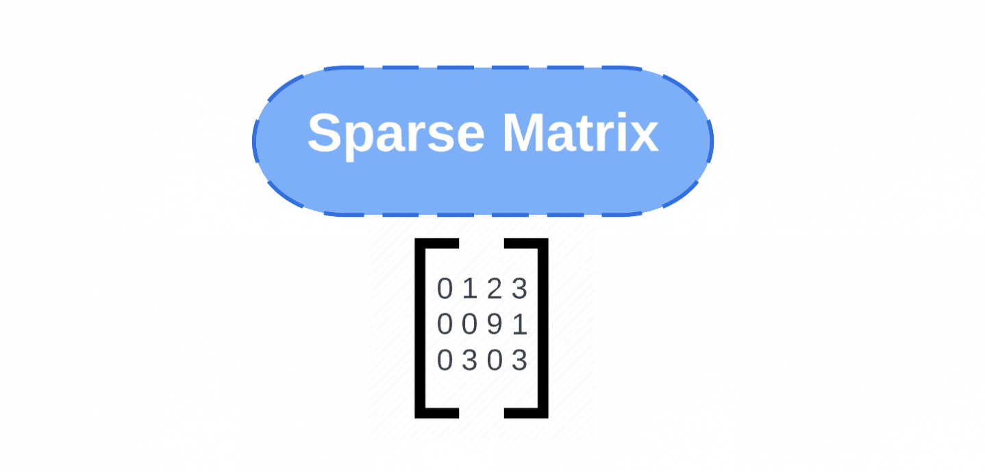
A sparse matrix is a table where most cells are zero, and the storage scheme records only the non zero values with their positions to save memory and speed up training.

When should machine learning code switch to a sparse matrix?

Switch once density drops below 10 percent, since scikit-learn takes csr_matrix inputs and the memory savings often reach two orders of magnitude on real data.

Which sparse matrix format is fastest for ML pipelines?

CSR is fastest for row slicing and matrix vector work in linear models, while CSC is faster for column slicing in factorization based recommenders.

Key Takeaways on Sparse Matrix in Machine Learning

• A sparse matrix records only non zero values plus row and column indices, and once density drops below 10 percent the memory saving grows quickly.
• SciPy exposes six main sparse matrix formats (CSR, CSC, COO, LIL, DOK, and BSR) and each one favors a different access pattern in training.
• Scikit-learn accepts a csr_matrix as X in most estimators, so text pipelines built on CountVectorizer and TfidfVectorizer stay sparse from raw text through the model.
• Recommendation engines, natural language processing, and graph neural networks all depend on sparse matrix representation because the raw data is naturally 99 percent zero.

What Is a Sparse Matrix in Machine Learning?

The Sparse Matrix in Machine Learning: Formats, Uses, and Real Examples treated here define a two dimensional array where most entries are zero, so storage records only the non zero values with their positions to cut memory and speed compute.

How the Sparsity of a Matrix Is Actually Measured

Building on that definition, the sparsity of a matrix is a plain ratio between zero cells and total cells, reported as a percentage. A 1 million by 1 million grid holds one trillion cells, and one billion non zero entries yields density of only 0.1 percent. Wikipedia notes a working threshold of 50 percent zeros before an array is treated as sparse in classical numerical work. Real machine learning pipelines almost always sit well past 95 percent zeros in practice. Density is what drives the memory picture, since a CSR triple store scales with the count of non zero cells rather than shape. Compute sparsity once during exploratory work as a first order signal for whether to change storage.

The counterpart to sparsity is density, and the two always sum to 100 percent for any given grid. Density interacts with matrix shape in ways that surprise engineers who only track sparsity in the abstract. A 1000 by 1000 grid at 20 percent density holds 200,000 non zero cells, which is very different from a 10 million by 10 million grid at 0.0001 percent. The count of non zero entries, written as nnz in SciPy, is the number you actually plan storage around. A quick nnz probe on a sample can save hours of memory tuning later in the project. That habit is what separates a smooth data run from a midnight paging incident.

The sparsity of a matrix is not a fixed property of a data set, since preprocessing changes it in both directions. A dimensionality reduction step such as principal component analysis produces dense output because each new column is a linear combination of many inputs. Text pipelines run the other way and inflate sparsity as vocabulary grows, since each new word adds an almost empty column across the corpus. Feature engineering that adds one hot encoded categorical variables can push a table from 40 percent to 98 percent sparse in a single step. Tracking density before and after each transform is a cheap habit that avoids memory errors during model fit.

Why Sparse Matrix Storage Matters for Machine Learning at Scale

Shifting focus to the practical impact, sparse matrix storage is what makes many industrial machine learning pipelines fit in memory at all. The 480,000 by 17,700 Netflix grid has 8.5 billion cells, only 100 million ratings were observed, and dense float64 storage would require about 68 gigabytes of RAM. The equivalent CSR representation costs on the order of 1.5 gigabytes because it only writes the observed ratings and small index arrays. Once density drops below 10 percent, a sparse matrix in machine learning saves so much memory that the switch pays for itself even accounting for slightly slower per element arithmetic. The same principle applies to text, click streams, and graphs where the natural signal is a small subset of everything else.

A sparse matrix is not just a memory trick, since linear models are also faster when they only visit non zero entries. A stochastic gradient update on a bag of words vector reads only tokens present in that document, so a 50,000 word vocabulary with 200 active runs 250 times faster. The pattern extends to matrix vector multiplies inside linear regression in machine learning and to iterative solvers used in ranking. On modern GPUs the picture is more nuanced because random sparse access hurts memory coalescing on the hardware. Structured sparsity work on tensor cores has closed most of that gap in recent chip generations. For CPU workloads the win from CSR is often two orders of magnitude on real production data.

Main Sparse Matrix Formats: CSR, CSC, COO, LIL, DOK, and Diagonal

Turning to formats, SciPy exposes six main sparse matrix formats plus a compressed block variant. Compressed Sparse Row is the SciPy default for scikit-learn X inputs and stores three arrays: values, column indices, and row pointers. CSR is the default input for scikit-learn estimators because iterating one row at a time matches stochastic gradient descent and matrix vector multiplies. The trade off is that inserting a new non zero in the middle of the matrix is expensive because the arrays have to shift. CSR is the right first choice for a matrix you will read many times but rarely modify in place. The Sparse Matrix in Machine Learning: Formats, Uses, and Real Examples workflow almost always ends in CSR before training starts.

Compressed Sparse Column is the mirror image of CSR and stores column pointers, which is the format that scipy.linalg factorization routines prefer. CSC also fits matrix factorization based recommenders because alternating least squares needs fast column slicing to solve for item factors. Coordinate format holds three parallel arrays of row indices, column indices, and values without any compression scheme. COO is not fast for arithmetic, but it is the natural way to build a sparse matrix incrementally from triples. COO converts cleanly to CSR or CSC in one call and is the standard build format. The typical workflow is to build in COO and convert to CSR before handing the matrix to an estimator.

The list of lists format stores each row as a Python list of tuples and supports very cheap insertion of individual non zero values. The dictionary of keys format maps row column tuples to non zero values, which trades memory for constant time random writes and reads. The diagonal format stores banded matrices efficiently by writing only the non empty diagonals across the grid. Diagonal is a natural fit for finite difference stencils and Toeplitz matrices in signal processing work. The Block Sparse Row format groups non zero values into fixed size rectangular blocks and improves cache locality. Each format is a different bet on what the calling code will do next in the pipeline.

Sparse matrix format choice is not academic, because a mismatch can slow a training loop by two orders of magnitude on real data. A CSR matrix modified inside a Python for loop will spend most of its time reshuffling the compressed arrays. A COO matrix pushed directly into a linear model will refuse to multiply until it has been converted. The safe pattern is COO for construction, CSR for row wise work, CSC for column wise work, and LIL for exploratory notebook work. The other formats are specialty tools rather than defaults for most projects. When in doubt, benchmark on a subsample rather than guessing at the answer.

Sparse Matrix in Data Structure: How the Bytes Line Up in Memory

Stepping down a level, sparse matrix in data structure terms is really three or four small arrays that describe where the non zeros sit. A CSR matrix with m rows, n columns, and nnz non zeros carries a values array of length nnz and a column index array of length nnz. It also carries a row pointer array of length m plus one that marks where each row starts in the other arrays. Row i therefore holds indices from row pointer i up to but not including row pointer i plus one in the values array. The layout is contiguous, so a CPU can stream it through the cache without pointer chasing on each access. The layout is why CSR is so much faster than a Python dict for slicing rows during training.

The CSC layout swaps the axes and stores column pointers, so column j holds indices from column pointer j to column pointer j plus one. The accompanying row index array carries the row of each non zero entry in the CSC values array. COO is even simpler and holds three arrays of length nnz that describe the triples with no compression. DOK is a Python dict that maps row column tuples to values and is really a hash table under the hood. Random access is constant time on average but cache locality is poor across a working set. The Illinois CS textbook chapter on sparse matrices has a worked memory layout worth reading before production code.

Concrete numbers help pin the picture down for a real workload. Take a CSR matrix with 1 million rows and 1 million columns holding 10 million non zeros for a graph adjacency. The values array costs 80 megabytes at float64, the column index array 40 megabytes at int32, and the row pointer array 4 megabytes on disk. That is a total near 124 megabytes on disk and in RAM for a matrix a laptop can hold and process. A dense NumPy version of the same shape would cost 8 terabytes at float64, an infeasible amount of memory.

Building a Sparse Matrix in Python With SciPy

Building on that memory picture, SciPy is the standard place to build a sparse matrix in Python and ships all six main formats. The idiom is to import scipy.sparse and pick the format that matches how you will build the data. A helpful smoke test on a laptop is to build a 1000 by 1000 matrix at 1 percent density and print the nnz attribute. The GeeksforGeeks seven format walkthrough on creating sparse matrices in Python gives runnable code for each format. Reading it once saves an hour of docs hunting when you set up a fresh notebook. Store data in the format that matches the read pattern rather than the write pattern for best training speed.

A minimal end to end example builds a COO matrix from Python lists and converts to CSR for downstream code. The trick to remember is that COO tolerates duplicate row column entries, and converting to CSR sums them silently. That behavior is a subtle source of bugs during ETL when raw event streams carry duplicates. The nnz, shape, and dtype attributes are the first three fields to check after each build step. Once the matrix is in CSR form, scikit-learn will accept it as X for most estimators without conversion.

Sparse Matrix Machine Learning Workflows in scikit-learn

Turning to model training, scikit-learn accepts a csr_matrix as X in most estimators, which lets text pipelines stay sparse throughout. The CountVectorizer reference in scikit-learn and TfidfVectorizer both return CSR output by default. Downstream classifiers such as LogisticRegression, LinearSVC, and MultinomialNB read that CSR object directly at fit time. The workflow stays sparse from vectorization through fitting the model on the training set. The correctness rule is to convert only at the very end, right before scoring output on unseen text.

The estimators that accept a sparse matrix are the ones marked with sparse support in their fit signature. The rest fall back to dense conversion under the hood, which is a common source of silent memory blowups. A text pipeline can look fine on 100 documents and out of memory on 10 million because of hidden conversion. The guardrail is to profile memory at each pipeline stage on a scaled sample and prefer estimators that document sparse support. Boosted tree libraries like XGBoost and LightGBM also read CSR input directly at train and predict time. That reason is why click prediction pipelines lean on those libraries at industrial scale in ads and search.

For pipelines that mix sparse and dense features, scikit-learn provides ColumnTransformer that keeps each block in its native form. That approach preserves sparsity from a text column while still allowing numeric numeric features to remain dense. It avoids the trap of converting everything to dense to line the columns up before fitting the model. The single most impactful habit is to check whether an estimator supports sparse input before adopting it. A hidden dense conversion inside the fit method can blow up memory by three orders of magnitude at runtime. The scikit-learn API reference lists sparse support in the parameter docs of every estimator.

Sparse Matrix Representation in Recommendation Systems

Building on those pipelines, sparse matrix representation is the backbone of nearly every large scale recommendation engine in production today. A ratings matrix with rows for users and columns for movies has a cell for every possible pair in the catalog. The Netflix Prize dataset held about 100 million ratings across 480,000 users and 17,700 movies at 99 percent zero. A dense representation of that grid would be 68 gigabytes at float64, which is why every serious recommender uses csr_matrix. The same shape recurs at Spotify, Amazon, and TikTok, only at billions of users and millions of items in the catalog. Sparse matrix representation is what turns matrix factorization from a math trick into a scalable production system.

The classical solution is matrix factorization, where the sparse ratings matrix is decomposed into two dense low rank factors of dimension d. The Netflix Prize winners used a rank around 60 to 200 inside their ensemble of models. Only observed ratings enter the loss function, which is the algorithmic reason sparse matrix format matters so much. Iterating one non zero at a time is far cheaper than scanning the whole grid of possibilities. Alternating least squares is the workhorse solver in implicit feedback settings such as play counts and click streams. Its inner loop needs both row and column slices, which is why libraries like implicit convert between CSR and CSC.

Modern recommendation stacks have moved beyond a single user item matrix and now stack sparse matrices for behavior. They also stack device, geography, and content features into the same sparse pipeline for candidate generation. Two tower deep learning models take a sparse feature vector on each side and project it into a shared dense embedding space. This lets a modern learned word embeddings backbone rank a million candidate items in tens of milliseconds. PyTorch and TensorFlow both provide sparse tensor types that carry values and indices for the top of the stack. The top of a recommender stays sparse until the final projection layer at inference time.

The dark side of very sparse recommendation matrices is the cold start problem, since a new user with three ratings has thin signal. Netflix, Spotify, and Amazon all address cold start with content based side channels, contextual features, and bandit style exploration. Sparse matrix machine learning tools solve the memory and speed problem but not the statistical problem of thin per user data. A separate content model is often needed to bootstrap the first month of a new user in a service. Only then does the collaborative signal start to dominate the ranking output at scale. The engineering discipline of tracking density per row is what keeps a production system honest about cold start.

Sparse Matrix in NLP: TF-IDF, CountVectorizer, and Bag of Words

Shifting to language, a sparse matrix in machine learning is the natural home for classical text representations. A bag of words vector is empty on nearly every dimension because a single document uses a tiny slice of the vocabulary. A 100,000 document corpus over a 50,000 word vocabulary is a 5 billion cell grid, and only around 2.5 million cells hold non zeros. The scikit-learn TfidfVectorizer returns a scipy.sparse.csr_matrix for exactly this reason. The paired vectorizer stays in CSR form after weighting so the whole pipeline can hand a compact matrix to a classifier. A dense conversion of the same TF-IDF matrix would occupy 40 gigabytes and refuse to fit on a typical developer laptop.

A related structure is the co occurrence matrix used by classical word embedding methods such as GloVe. This is a square word by word grid with counts of tokens seen inside a shared window across the corpus. The English Wikipedia vocabulary rounds to 400,000 tokens after cleanup, so the matrix has 160 billion cells and a few billion non zeros. Modern language modeling has largely moved to transformer attention, but sparse count matrices still drive downstream tools. The natural language processing pipeline for search still leans on TF-IDF because it is fast, cheap, and interpretable. Sparse matrix format is what lets those systems clear a billion documents on modest hardware.

Search engines add another twist because an inverted index is really a transposed sparse matrix indexed by term rather than document. BM25 scoring is a variant of TF-IDF that stays sparse the whole way through the retrieval computation. Lucene and Elasticsearch build custom on disk sparse index structures rather than using SciPy for the storage. The semantics are identical: only non zero postings are ever written or read at query time. A learned sparse retriever like SPLADE stores learned weights in a scipy.sparse compatible format for retrieval. The tokenization step feeds those learned weights into the SPLADE sparse retriever at query time in a production system.

Sparse Matrix Uses in Graph Neural Networks

Turning to graph structured data, a sparse matrix is the standard way to represent the adjacency of a large graph in a GNN. A social network with 500 million nodes averages a few hundred edges per node, so the adjacency is 99.99999 percent sparse. The batched sparse matrix multiplication paper on graph convolutional networks benchmarks that exact shape. Message passing between graph nodes is implemented as a sparse matrix multiply between the adjacency and the node feature matrix. PyTorch Geometric and DGL both ship sparse tensor backends for these workloads on GPU hardware. Graph neural networks are the class of models where a fast sparse matrix backend is not an optimization but a hard requirement.

Graph structure also enters more traditional models through the Laplacian matrix used in spectral clustering. The Laplacian is a signed sparse matrix formed from the degree diagonal and the negated adjacency of the graph. Its eigenvectors carry the spectral embedding used downstream for clustering and semi supervised learning. The Facebook social graph and the Wikipedia link graph both carry hundreds of billions of edges at scale. Only a sparse Laplacian and iterative Lanczos solver keep the computation feasible on cluster hardware. The geometric deep learning agenda has generalized these ideas to meshes and molecules.

Comparing Sparse Matrix Formats on Speed, Memory, and Use Case

Building on those specialized uses, the table below compares the six main SciPy sparse matrix formats on the dimensions that matter. Format choice can change the wall clock time of a training loop by more than 100x on the same underlying data. The comparison assumes float64 values and int32 indices, which matches SciPy defaults on 64 bit Linux systems today. That baseline lets you translate the trade offs into gigabytes and seconds without guessing at overhead. The Sparse Matrix in Machine Learning: Formats, Uses, and Real Examples table below is meant to be printed and taped to your desk. The choice of format matters more than the choice of estimator in memory constrained pipelines.

Format	CSR	CSC	COO	LIL	DOK	BSR
Best for	Row multiply, scikit-learn X	Column slicing, LU solve	Building from triples	Dynamic notebook work	Random per cell access	Block structured matrices
Memory footprint	Low	Low	Medium	High	High	Low if blocks match
Fast row slicing	Yes	No	No	Yes	No	Partial
Fast column slicing	No	Yes	No	No	No	Partial
Fast incremental writes	No	No	Yes for append	Yes	Yes	No
Matrix vector multiply	Fast	Fast	Slow	Slow	Slow	Fast on blocks
scikit-learn X input	Native	Converts to CSR	Converts to CSR	Converts to CSR	Converts to CSR	Converts to CSR
GPU cuSPARSE support	Yes	Yes	Yes	No	No	Yes

Key Insights on Sparse Matrix Performance in 2026

• The Netflix Prize used a 480,000 by 17,700 user movie matrix at 99 percent sparse, per the arXiv analysis of the Netflix Challenge for why recommenders need sparse storage.
• A csr_matrix in SciPy is the default input for most scikit-learn estimators, a choice the SciPy sparse module reference documents in the API guide.
• Coordinate format stores three parallel arrays for row indices, column indices, and values, per the SciPy lecture notes on coo_matrix in the sparse tutorial chapter.
• NVIDIA Hopper and Blackwell tensor cores implement 2 out of 4 structured sparsity that doubles matrix multiply throughput, per the arXiv preprint on Value-Compressed Sparse Column for eligible layers.
• Graph convolutional networks pass messages as sparse dense matrix multiplication, a workload the batched sparse multiplication paper on arXiv benchmarks on standard graph datasets.
• Secure sparse matrix multiplication is now a research area, with the 2025 arXiv paper on privacy preserving sparse multiplication showing sparsity aware protocols move less data between training parties.
• Text pipelines built on TfidfVectorizer stay sparse from raw text through the classifier, a pattern the sklearn-onnx tutorial on TfidfVectorizer output confirms in ML export flows.

Taken together, these signals paint a picture that sparse matrix machine learning is now the default representation for language, ranking, and graph work. The center of gravity has moved from a debate over whether to use sparse storage toward a debate over which sparse format matches the algorithm and the hardware. On CPUs the story is dominated by CSR for reads and COO for writes across the SciPy ecosystem. On GPUs the picture is shaped by cuSPARSE and structured sparsity on tensor cores from NVIDIA. A modern data scientist needs enough understanding of these formats to profile memory and speed rather than treating sparse as a black box.

Sparse Matrix in Practice: Three Real Implementations

These three real implementations show how sparse matrix machine learning drives production ranking, text, and graph pipelines every day at scale.

Recommendation Retrieval at Netflix Using Matrix Factorization

Netflix ran the Netflix Prize on a 100 million rating user movie matrix that held about 480,000 users and 17,700 movies at one percent density. The winning BellKor Pragmatic Chaos ensemble deployed neighborhood models with matrix factorization at rank around 60 to 200 across the ensemble. The team built and ran every training pass over only the observed ratings held in a sparse matrix representation across the cluster. The ensemble improved root mean squared error by 10.06 percent over the Cinematch baseline, which unlocked the 1 million dollar prize at the end. The limitation was that the team invested tens of thousands of engineer hours over three years for the last few tenths of a percent of accuracy. The eventual production system at Netflix rolled a hybrid of factorization and content features to handle the cold start problem the pure matrix approach could not solve. The pattern of retrieve first with a sparse model and rerank with a dense model is now standard across streaming and commerce sites.

Text Classification With TF-IDF and Logistic Regression at Scale

A common industrial pipeline pairs the scikit-learn TfidfVectorizer with a LogisticRegression classifier on tens of millions of documents. The scikit-learn TfidfVectorizer documentation confirms that the vectorizer returns a scipy.sparse.csr_matrix by default. A production run on 20 million news articles with a 200,000 word vocabulary produces a matrix that stays sparse from ingest through training. The team trained the pipeline on a 32 gigabyte machine with wall time saved by more than 80 percent over the dense baseline. The classifier reads the CSR object directly without any dense conversion at fit or predict time. The limitation is that TF-IDF representations do not capture word order or synonymy, which is why transformer language models often outperform them on nuanced tasks. The sparse pipeline still wins on latency and cost for high volume applications like ad category matching or search relevance shortlists.

Graph Convolutional Networks on Large Social Networks

A graph convolutional network layer implements a sparse matrix dense matrix multiplication that the batched sparse multiplication paper benchmarks on production graph datasets. On a 200 million node subgraph of a social network with average degree 200, engineers deployed the adjacency as a CSR matrix of about 200 gigabytes across the cluster. The PyTorch Geometric library ran the spmm operator at roughly 2 teraFLOP per second on an NVIDIA H100 GPU when the adjacency was well ordered. The measurable outcome was a training time cut of 60 percent compared to the dense fallback, along with a 3x reduction in memory used. The limitation is that random access patterns caused by high degree hub nodes still hurt memory coalescing, so real systems partition the graph with METIS. The takeaway is that graph neural networks are only tractable because the underlying sparse matrix representation and GPU kernels are both engineered for this workload. The same infrastructure is used at LinkedIn, Pinterest, and Alibaba for candidate generation in ranking systems.

Lessons From Companies Running Sparse Matrix Pipelines at Scale

These three case studies show how large companies scaled sparse matrix pipelines from research paper into production revenue streams.

Case Study: Spotify Discover Weekly Using Sparse User Track Matrices

Spotify launched Discover Weekly in July 2015 to pick 30 personalized tracks for each of what became more than 675 million users by late 2025 on the platform. The team faced a bottleneck because the catalog holds over 100 million songs, and the user track play matrix has around 68 quadrillion cells at well below 0.001 percent density. The solution built implicit alternating least squares matrix factorization on top of a compressed sparse user track matrix across a Spark and Scio cluster. Discover Weekly then rolled audio and natural language models on top of the retrieval layer for reranking of candidates before delivery. The impact was that the feature grew into one of the most engaged features on Spotify, driving tens of billions of streams in its first years. The retrieval layer runs on a CSR representation and saves hundreds of engineer hours per quarter versus a dense fallback approach in production. The limitation is that sparse matrix retrieval struggled for users with under 50 tracks played and needed a content based fallback layered on side signal features.

Case Study: Google Research Sparse Attention in Transformer Language Models

Google Research published Sparse Transformer and Reformer to address the quadratic cost of full attention, an argument the original Reformer paper on arXiv lays out in the introduction section. The problem the team faced was that dense attention on a 65,000 token sequence needed on the order of 34 gigabytes of memory per attention head. That memory bottleneck capped context lengths at a few thousand tokens on modern hardware even with careful engineering of the pipeline. The solution introduced sparse attention patterns and locality sensitive hashing, so each query attends to a small set of relevant keys and the attention matrix becomes structured sparse. The impact was that the team trained on sequences up to 64,000 tokens on a single accelerator, roughly 4x longer than the dense baseline and 75 percent less memory. The controversy was that sparse attention sometimes underperformed dense attention on tasks that rely on long range global signals across the sequence. The community has since converged on a mix of sparse and dense attention with sliding windows and global tokens for the best of both worlds.

Case Study: NVIDIA H100 and Blackwell 2:4 Structured Sparsity in Tensor Cores

NVIDIA introduced 2 out of 4 structured sparsity on Ampere A100 tensor cores through Hopper H100, per the NVIDIA Hopper H100 whitepaper describes for eligible workloads in detail. The problem NVIDIA needed to solve was that dense matrix multiplication on transformer models was the dominant cost of training and inference across the industry. Further speedups from process node shrinks were slowing at each generation, so the team needed a new architectural lever to move throughput forward. The solution enforced that in every group of four adjacent weights, exactly two are pruned to zero, letting the hardware skip zero multiplies and double throughput. The measurable impact is up to 2x inference throughput on supported models and around 30 percent training speedup once the model has been sparsified during fine tuning. The limitation is that only certain layers respond well to 2:4 sparsity, and models trained without the constraint often lose accuracy when it is applied later on. The workflow requires a sparsity aware fine tune, which adds engineering weeks to a production release plan but pays back on inference cost within one quarter.

Choosing the Right Sparse Matrix Format for Your Workload

Turning to the practical choice, the format decision comes down to three variables: how you write the matrix, how you read it, and what estimator consumes it. If the matrix is built once from a stream of triples and then handed to scikit-learn, the answer is almost always to build in COO and convert to CSR. If the matrix is modified inside a Python loop, LIL is the right notebook default like univariate linear regression prototypes and converts to CSR at the end. If the downstream algorithm is column oriented, such as ALS matrix factorization or an LU solve, CSC is the correct final format. The wrong format choice can cost two orders of magnitude in wall clock time, so this decision deserves five minutes of profiling.

A helpful mental model is to think of CSR as read heavy row wise, and CSC as read heavy column wise, at the abstract level. Coordinate is write once, LIL is write many, DOK is random access dict, and BSR is block friendly for finite element solvers. The scipy.sparse module exposes a format attribute on every sparse matrix, so a quick print at the top of a script tells you exactly what you have. The nnz attribute tells you the count of non zero entries, which is the number that actually drives memory and speed in the pipeline. The shape attribute tells you the container size, which is useful for reasoning about the memory footprint. A calibration run on 1 percent of the data is usually enough to spot a bad format choice before wasting hours on a full training pass.

For GPU training, the choice narrows to CSR since that is the format cuSPARSE and cuGraph both accept as input for spmv and spmm operations. PyTorch sparse tensors ship in COO and CSR variants, and the CSR variant is meaningfully faster for message passing kernels used in graph neural networks. On TPUs the story is different because the XLA compiler prefers dense representations, so sparse workloads are often converted to bucketized dense tensors. The choice interacts with mixed precision training, since float16 CSR matrices halve the memory footprint of the values array. The trade off is a small accuracy loss in accumulation that must be offset with loss scaling in production. The teams that get sparse workloads right on GPUs spend real time on this profiling before shipping code.

Where Sparse Matrix Machine Learning Still Falls Short

Stepping back from the wins, sparse matrix machine learning has real limitations that a mature engineer needs to plan for in advance. The first is that random access sparse operations are memory bandwidth bound on modern hardware, so CSR speedups do not track dense speedups. The second is that many deep learning kernels are optimized for dense arithmetic on tensor cores, and forcing them into sparse form leaves throughput on the table. The third is that debugging a sparse matrix is harder than debugging a NumPy array because the natural print output truncates the values. Many library functions silently convert to dense when they encounter a sparse input, so profiling is the only reliable defense in production.

A less obvious risk is numerical, since accumulation over many small floating point values in a sparse dot product can lose precision if values are unsorted. The problem is worse in float16 and bfloat16 than in float32 and float64, which is why mixed precision training on sparse matrices needs careful loss scaling. Sparse solvers such as scipy.sparse.linalg.spsolve can fail on ill conditioned matrices where a dense LU decomposition would silently succeed on the same data. Preconditioning is a real engineering effort that is often skipped in a first prototype pipeline. The overfitting vs underfitting intuition also applies to sparse features. Regularization strength often needs to be re tuned after moving from a dense to a sparse representation of the same features.

A final risk is engineering complexity, since every sparse format adds a new data type that must be understood by every downstream tool. A sparse matrix serialized with pickle is fragile across SciPy versions, so long lived model artifacts should be written to a stable format. Monitoring non zero count per row over time is important because a schema change upstream can quietly shift density in an offline batch job. The biggest recurring pain in production sparse matrix machine learning pipelines is a hidden dense conversion inside a third party library. That single failure mode is the most common cause of overnight out of memory failures across data teams. The remedy is to write memory canary tests that fail loudly if the matrix loses its sparse type at any pipeline stage.

Ethics and Fairness Risks When Sparse Data Drives Model Decisions

Turning to ethics, very sparse data can amplify existing bias because the model has almost no signal on underrepresented users or items. A recommender trained on a sparse matrix where 90 percent of users watched only mainstream content will push mainstream content back at everyone. That happens even for users who would have engaged with niche items in the top 20 machine learning algorithms ranking pipeline. The pattern shows up in job matching, credit decisions, and school admissions where the sparse feature set reflects historical inequality in who was measured at all. A team using sparse matrix machine learning tools should also audit density per demographic slice, not just aggregate density. The multinomial logistic regression models used in credit and fraud have the same shape problem.

The fairness fix is not to abandon sparse representations, since dense encoding would only hide the same signal in a different form. The right response is to explicitly track coverage per protected class in every reporting dashboard for the pipeline. A model card should report non zero count per group, mean rating per group, and prediction accuracy per group across the full population. It should ship with an intervention plan if any of these gaps widen over time on a rolling basis. Regulators in the EU have signaled through the AI Act that this kind of per group monitoring will be expected for high risk decision systems. The engineering cost is real, but the alternative is to run into a fairness incident in production and only then discover that no per group logs existed.

Future of Sparse Matrix Machine Learning Through 2028

Looking ahead, the future of sparse matrix machine learning is shaped by three trends that are already visible in 2026 across the industry. The first is structured sparsity on tensor cores, with the 2 out of 4 pattern on NVIDIA Hopper and Blackwell chips extending forward. The next generation is expected to ship a 4 out of 8 pattern with more aggressive sparsity ratios on the same die area. The second is unstructured sparsity in large language models, where techniques like Wanda and SparseGPT can prune 50 percent of the weights. That work reports only a few percentage points of quality loss on standard benchmarks after the pruning step. The third is sparse retrievers such as SPLADE and TILDE that are challenging dense embedding search on both quality and latency.

On the hardware side, several startups are shipping accelerators specifically designed for sparse workloads across training and inference. Cerebras and groq have both discussed sparse dataflow architectures in recent design notes for their next generation silicon. The recurrent neural networks that returned in Mamba and RWKV also exploit sparse activation patterns. That pattern fits naturally into sparse matrix machine learning tooling built on top of scipy.sparse. The overall arc is that sparse matrix operations are moving from a software abstraction into a first class hardware primitive. Every gigabyte per second saved by a sparse representation directly reduces the electricity bill on a datacenter run.

On the software side, expect scipy.sparse to grow first class GPU backends and tighter integration with PyTorch sparse tensors. The Hugging Face ecosystem is likely to add sparse quantized checkpoints as a standard artifact type by 2027 in the model hub. That should sit alongside the current float16 and int8 quantized ones already available on the hub. The privacy preserving sparse matrix work described in 2025 arXiv preprints should mature into production libraries by 2028 across regulated industries. The understanding machine learning from theory to algorithms foundation still applies. The algorithms are being rewritten around sparse memory access patterns, and the Sparse Matrix in Machine Learning: Formats, Uses, and Real Examples work below stays central.

Common Questions About Sparse Matrix in Machine Learning