Autoencoders

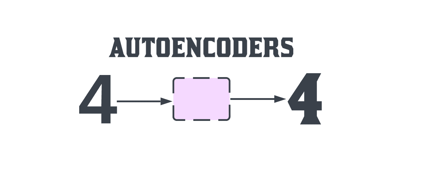
Introduction

Autoencoders sit at the quiet center of modern machine learning. They power anomaly detection systems, image denoisers, recommendation pipelines, and the latent spaces of diffusion models that generate today’s viral images. A 2025 Springer review of deep autoencoder networks catalogued more than four hundred production and research applications across engineering, biomedicine, and finance in a single year. The core idea has stayed simple since Hinton popularized it, yet the architecture has quietly become the workhorse behind representation learning at scale. This guide walks through what they are and how the encoder decoder architecture actually works. It also covers complete versus undercomplete configurations, every major type in current use, and the limitations of these models that practitioners hit in production. It also connects the classical picture to how modern basics of neural networks feed into today’s foundation models. Read straight through for a theory-first tour, or jump to the sections that match the search intent that brought you here.

Quick Answers on Autoencoders and How They Work

What are autoencoders in machine learning and how do they compress data effectively?

Autoencoders are unsupervised neural networks that learn to compress input into a small latent code and reconstruct the original from that code. The bottleneck forces the network to keep only the most useful features.

What is the autoencoder architecture in one straightforward line for practitioners?

Autoencoders use a three block encoder decoder architecture that trains without labels. The encoder shrinks input to a bottleneck code, then the decoder expands the code back to the original space during reconstruction.

What are the main limitations of these models that teams hit in production?

Autoencoders overfit small datasets, produce lossy reconstructions, need careful bottleneck sizing, and yield latent spaces that are hard to interpret without extra probes or regularization.

Key Takeaways

• Autoencoders compress input to a latent code and reconstruct it, learning features without labels.
• Complete, undercomplete, and overcomplete refer to the size of the bottleneck relative to the input.
• Denoising, sparse, contractive, and VAEs each add a constraint that shapes what the latent code learns.
• Limitations of these models include overfitting, lossy reconstruction, opaque latents, and heavy compute at scale.

What Is an Autoencoder in Simple Terms

Autoencoders are self supervised neural networks that compress input to a compact latent code and rebuild the original from that code. The bottleneck forces the network to keep only the features useful for reconstruction.

That framing lets teams train useful representations on data that has no labels, which is most enterprise data. Practitioners then reuse the encoder as a feature extractor for downstream tasks like clustering, retrieval, anomaly scoring, or supervised fine tuning. The supervised or unsupervised deep learning question has a firm answer for autoencoders. For autoencoders the answer is unsupervised or self supervised, depending on the exact training regime used by the team. This is what makes them attractive for pretraining, feature extraction, and anomaly detection on messy real world data.

The core intuition behind autoencoders is simple to state in one line. If a network can rebuild an image from a hundred numbers, then those hundred numbers must summarize the image. That summary is called the latent representation, and the whole point of the autoencoder is to shape it. A well trained autoencoder produces a latent code smoother, smaller, and more useful for downstream tasks than the raw input. The classic three block picture also gives you a concrete way to visualize the reconstruction loss during training. Understanding the reconstruction target frames every design choice that follows.

How to Implement the Autoencoder Architecture End to End

Building on that plain description, the autoencoder architecture always has three visible pieces: encoder, bottleneck, and decoder. The encoder is a stack of layers that shrinks the input. The bottleneck is the smallest layer where the compressed code lives, and the decoder is a mirror stack that expands the code back out. The classic autoencoder architecture explained by APXML shows this three block shape in every canonical diagram since the 1980s. Everything else about the model is a variation on those three blocks. Understanding the three block skeleton first makes the variants far easier to follow.

The encoder is usually a set of dense or convolutional layers with nonlinear activations between them. Each layer projects the input into a smaller space, so a 784 pixel MNIST image might pass through 512, 256, and 128 units before reaching the bottleneck. Convolutional variants replace the dense layers with convolution and pooling, which respect the spatial structure of images. The choice of activation function shapes the smoothness of the latent code and matters for whether the network can be interpreted later. Practitioners typically pick ReLU or GELU with batch normalization between layers.

The bottleneck is where the interesting learning happens because it is the physical constraint that forces compression. If the bottleneck is smaller than the input, the encoder cannot memorize every pixel and must learn shared structure. If the bottleneck is larger than the input, the network can cheat by copying values through unless it is regularized. The size of the bottleneck is one of the most sensitive hyperparameters in the entire model, and getting it wrong is a common failure mode. A useful debugging habit is to plot reconstruction loss at several bottleneck sizes and pick the elbow.

The decoder mirrors the encoder so the output has the same shape as the input, which lets the loss function compare the two directly. In dense variants the decoder is a set of layers that grows the code back up through 128, 256, 512, and 784 units. In convolutional variants the decoder uses transpose convolutions or upsampling to rebuild the spatial map. The last layer of the decoder is usually a linear or sigmoid layer whose activation matches the input distribution. Matching the last activation to the input distribution is the small but important step that lets the loss function stay well behaved during training.

Encoder, Bottleneck, and Decoder in Detail

Turning to the three blocks in more depth, each one plays a specific role that the others cannot replace. The encoder chooses which features survive compression during the forward pass through every layer. The bottleneck decides how much information can pass through, and the decoder decides how faithfully the code can be turned back into the input. The Towards Data Science introduction to autoencoders breaks the same three roles into a helpful diagram. Treating the three blocks as separate objects rather than one monolithic model makes debugging and comparison much easier. Every failure mode we discuss later maps neatly to one of these three blocks.

A convenient way to think about the bottleneck is as a controlled information channel with limited capacity. If the input has 784 dimensions and the bottleneck has 32, no more than 32 continuous numbers can describe the image. The reconstruction has to be built entirely from those numbers, which is what forces the model to learn general features rather than pixel level noise. This capacity constraint is why undercomplete networks learn useful features and why overcomplete networks need regularization to do the same. Any change to the bottleneck therefore has an outsized effect on downstream tasks like clustering or anomaly scoring.

The decoder rarely gets as much attention as the encoder, yet its capacity shapes what the encoder is allowed to learn. If the decoder is too weak, the encoder cannot store subtle features because they cannot be rebuilt. If the decoder is too strong, it can hallucinate details that were never in the code, which hides reconstruction errors that matter. Practitioners often use symmetric encoder and decoder capacity as the safe default and only deviate for specific reasons. Careful decoder design is especially important for medical imaging and defect detection where hallucinated details would mislead reviewers.

Complete, Undercomplete, and Overcomplete Autoencoders

Stepping back to the whole family, the three configurations of complete, undercomplete, and overcomplete networks differ only in the size of the bottleneck relative to the input. An undercomplete autoencoder has a bottleneck smaller than the input, so the network is forced to compress and learn general features. An overcomplete autoencoder has a bottleneck larger than the input, so it can copy values through unless a regularizer stops it. A complete autoencoder has a bottleneck equal in size to the input, which lets it in principle memorize the input perfectly. The APXML explainer on undercomplete and overcomplete networks lays out this taxonomy in a single diagram.

Undercomplete they are the default choice for dimensionality reduction and are the closest relative of principal component analysis. A linear undercomplete autoencoder with a mean squared error loss actually learns the same subspace as PCA when trained to convergence. Nonlinear encoders make the model strictly more expressive and let it capture curved manifolds that PCA cannot see. This is why teams reach for undercomplete networks when they want feature vectors for clustering, retrieval, or downstream classification. The bottleneck size becomes a lever that trades reconstruction fidelity against downstream usefulness.

Overcomplete autoencoders sound counterintuitive because a larger bottleneck seems to defeat the whole point of compression. The catch is that the extra units are only useful if a regularizer prevents the identity map from being learned. Sparse autoencoders, denoising variants, and contractive they are all common ways to regularize an overcomplete network so it learns meaningful features. Without regularization an overcomplete network usually collapses to a trivial copy that memorizes and generalizes poorly. Practitioners often reach for overcomplete networks when they need rich features for anomaly detection or transfer learning.

A complete autoencoder sits in between and is rarely used in production because it can memorize without learning. The complete autoencoder definition that gets searched from Google is essentially this. A complete autoencoder has a bottleneck the same size as the input, which allows perfect reconstruction in principle but not useful features. In tutorial contexts it appears as a stepping stone that shows why compression matters. Once you have written a complete autoencoder and watched it memorize, the value of the undercomplete and regularized overcomplete variants becomes obvious. Complete they remain useful as a debugging tool for verifying that a training loop is set up correctly.

Training Loss Functions and Optimization Signals

Moving on from architecture choices, the loss function is what tells the network whether its reconstruction is good enough. Mean squared error is the classic choice for continuous inputs like grayscale images or tabular features. Binary cross entropy is the standard when the input is a probability or a binary image, and it aligns cleanly with a sigmoid output layer. Categorical cross entropy shows up when the input is a one hot encoding, though this is less common in autoencoder work. Understanding the pairing between output activation and loss is essential and is covered well in our cross entropy loss in machine learning primer.

Beyond the base reconstruction term, most modern variants add regularization terms that shape the latent code. Sparsity penalties push individual activations toward zero so only a few units fire per input. KL divergence terms push the aggregate latent distribution toward a target prior, which is the core idea behind VAEs. Contractive penalties push the Jacobian norm down so small input changes produce small latent changes. The mix of terms in the loss function is often what distinguishes one autoencoder variant from another, and small changes can have large behavioral effects.

Optimization itself is mostly Adam or AdamW with a cosine or step schedule, but a few autoencoder specific choices matter. Gradient clipping helps for very deep autoencoders where transposed convolutions can produce large gradients late in training. Batch normalization or layer normalization between encoder blocks stabilizes the latent distribution and speeds up convergence. Our post on how batch normalization accelerates training covers the mechanics in more detail. Practical training also benefits from early stopping on a held out reconstruction loss to prevent overfitting.

Denoising Autoencoders and Their Role in Robust Feature Learning

Shifting to the individual types of these models, denoising they are the variant that made this whole family famous in modern deep learning. A denoising autoencoder is trained on inputs that have been deliberately corrupted with noise, but the target is the clean original. The corruption forces the encoder to learn features that survive noise, which usually means features that describe global structure rather than pixel level detail. The E2E Networks explainer on denoising variants shows how salt and pepper noise or Gaussian noise reshape the reconstruction task. This training trick alone often turns a mediocre autoencoder into a strong feature extractor for downstream tasks.

Denoising these models show up in two big practical settings across the wider deep learning ecosystem today in enterprise pipelines. The first is signal cleanup, where the model directly rebuilds a clean image, audio clip, or sensor reading from a noisy input. The second is pretraining, where the encoder learned during denoising is repurposed as a feature extractor for a downstream classifier or detector. The pretraining use case anticipates how masked language models like BERT would later be built, because both approaches train on a corruption plus reconstruction objective. That conceptual lineage is one reason denoising they remain worth studying even in the transformer era.

Sparse Autoencoders and the Push for Efficient Representations

Building on that lineage, sparse variants regularize the latent code so only a few units fire for any given input. Sparsity is enforced by adding a penalty term to the loss, usually an L1 term on activations or a KL divergence against a small target activation probability. The result is a code where each unit specializes in a specific feature and inactive units stay quiet. Sparse autoencoders come up in the current interpretability wave because that specialization makes it easier to name what each unit represents. Anthropic and OpenAI research teams have used sparse variants to probe the internal features of large language models throughout 2024 and 2025.

The classic use of sparse variants is feature extraction on high dimensional data where a dense code would be hard to interpret. In fraud detection, a sparse latent code often maps to distinct behavioral patterns like new device sign in, unusual amount, or unfamiliar merchant category. Anomaly detection benefits because a rare input tends to activate an unusual combination of the sparse units. This makes the latent code both compact and legible, two properties that dense codes rarely combine. Practitioners tune the sparsity coefficient carefully because too much sparsity kills reconstruction quality.

Sparse autoencoders also connect neatly to the study of biological neural coding, where a small fraction of neurons fire for any given stimulus. The biological connection helped motivate the original sparse coding literature by Olshausen and Field in the late 1990s. Modern implementations rediscover the same result: sparse codes generalize better and transfer more cleanly across tasks. This is why the technique keeps returning in new forms every few years even as dense architectures dominate other areas. If you are new to sparse coding, our PyTorch loss functions primer is a good starting point for the L1 penalty implementation.

Contractive Autoencoders and Local Stability of Features

Turning from sparsity to smoothness, contractive variants add a penalty that keeps the latent code stable under tiny input changes. The added term is the Frobenius norm of the Jacobian of the encoder activations with respect to the input. That penalty pushes the encoder to produce very similar codes for very similar inputs, which is what stability means in this context. Contractive they are the smoothness cousin of sparse and denoising variants, and all three add a term that shapes the latent geometry. Their outputs are less flashy than denoising or variational variants, but they matter in industrial applications where noise is small but continuous.

Where you actually see contractive variants is in sensor networks and industrial monitoring where readings drift constantly. A small change in temperature or pressure should produce a small change in latent code, not a jump. Without the contractive penalty, standard these networks can produce jumpy latents that trigger false anomaly alarms for readings that are still inside normal operating ranges. That failure mode is expensive on a factory floor because false alarms erode operator trust in the model. Contractive regularization mitigates the problem without changing the overall architecture, which is why it is a favorite of process engineering teams.

Variational Autoencoders and Probabilistic Latent Spaces

Moving to the most influential variant, VAEs replace the deterministic latent code with a probability distribution over latents. Instead of predicting a single vector, the encoder predicts a mean and a variance that define a Gaussian distribution in latent space. The decoder samples from that distribution and rebuilds the input, and a KL term keeps the distribution close to a standard normal prior. This probabilistic setup means the latent space is smooth and interpolatable, which is what makes VAEs useful as generative models. The TechTarget definition of VAEs walks through the reparameterization trick that makes training possible.

Variational autoencoders were introduced by Kingma and Welling in 2013 and quickly became the standard way to think about learned generative distributions. The mean and variance framing gives you a principled way to sample new examples, interpolate between existing ones, and measure how surprising a new sample is under the learned distribution. Anomaly detection systems built on VAEs exploit that measurement directly by flagging samples whose latent probability is low. In generative art contexts you can walk through the latent space to produce smooth visual transitions that pure these networks cannot match. The same conceptual toolkit later informed the design of latent diffusion.

The main practical issue with VAEs is the tradeoff between reconstruction fidelity and latent smoothness. A stronger KL term produces smoother latents but blurrier reconstructions, and a weaker KL term produces sharper reconstructions but rougher latents. Teams often use annealed schedules that start with a small KL weight and increase it as training progresses. Beta VAE variants make this tradeoff explicit through a single hyperparameter that scales the KL term. Related concepts appear in the family of generative adversarial networks, which trade probabilistic clarity for sharper samples.

Modern VAEs are also the backbone of latent diffusion models like Stable Diffusion, where the VAE compresses images into a small latent space before diffusion runs. This is why VAEs matter far beyond their classic role in unsupervised learning. Almost every recent open image generator uses a pretrained variational autoencoder to reduce the cost of the diffusion pass. That means understanding VAEs is now a practical requirement for anyone building or auditing image generation systems in the current generative AI wave. Teams that skip VAE literacy end up with brittle pipelines because they miss the compression layer that shapes everything downstream.

Convolutional and Deep Autoencoder Variants

Shifting from probabilistic to structural variants, convolutional and deep autoencoders extend the base architecture in two orthogonal directions. A convolutional autoencoder replaces the dense encoder and decoder with convolution and transpose convolution layers, which respect the spatial structure of images. A deep autoencoder stacks many layers to increase capacity and depth without changing the fundamental block shape. Both variants improved reconstruction quality on natural images by large margins over dense networks. Convolutional autoencoders are the standard choice for medical imaging, remote sensing, and computer vision pipelines where spatial hierarchies matter.

Deep autoencoders bring their own operational and training complications for teams pushing into more than a handful of layers. Very deep dense variants suffer from vanishing gradients and are hard to train without careful initialization and normalization. Skip connections between encoder and decoder blocks help gradients flow, which is the origin of the U Net architecture that dominates medical segmentation. Our earlier post on how image recognition works touches on the same convolutional patterns that underpin these models. In practice most autoencoder deployments in industry are convolutional or hybrid rather than purely dense.

Recent variants combine convolutional encoders with transformer decoders or vice versa, blurring the boundary between autoencoders and modern sequence models. These hybrids show up in speech, time series, and video applications where local and global structure both matter. Related sequence models are covered in our recurrent neural networks explained guide for readers who want the sequence context. Practitioners increasingly treat the encoder and decoder as building blocks that can be swapped freely rather than as a fixed architecture. The result is a much richer design space than the classic three block picture suggests.

Autoencoders in Practice Across Industry Domains

Beyond the taxonomy, these models show up wherever teams need to compress, denoise, or score data without labels. Anomaly detection in banking uses reconstruction error to flag transactions that the model cannot rebuild well, which usually means unusual behavior. Medical imaging teams use denoising and convolutional variants to clean scans and to pretrain feature extractors for downstream diagnosis models. Recommendation systems use autoencoders to learn latent embeddings of users and items that power collaborative filtering. The variety of use cases is the reason they remain a first choice tool for representation learning across industries.

Manufacturing and industrial operations are another heavy user because sensor data is plentiful but rarely labeled. A contractive or denoising autoencoder trained on normal sensor traces from a machine can flag deviations long before a failure. Predictive maintenance teams often pair autoencoder reconstruction error with a rule engine that decides when to raise a maintenance ticket. The Viso deep dive on autoencoder applications catalogs several manufacturing case studies including a paper mill deployment that cut downtime by double digit percentages. These wins are why autoencoders are quietly embedded in more industrial systems than any other neural network family.

Autoencoders are also becoming a fixture inside generative pipelines even when they are not the star of the show. Latent diffusion models compress images through a variational autoencoder before running the diffusion process, which cuts compute cost by an order of magnitude. Audio generation systems use autoencoders to compress waveforms into small tokens that a language model can then predict. Even large language model interpretability work uses sparse variants to probe hidden states. The shared theme is that autoencoders are the workhorse for compression whenever a downstream model needs a small usable representation.

Where Autoencoders Fall Short and the Real Risks in Production

Turning to the honest tradeoffs, the limitations of these models are the reason so many production systems augment them with rule engines or supervised classifiers. Autoencoders overfit when the training set is small relative to model capacity, and the overfit shows up as memorization rather than generalization. Reconstruction is inherently lossy, so any downstream task that needs pixel level accuracy must compensate. The TechTarget troubleshooting guide on autoencoder limitations lays out eight practical limitations that map cleanly to production failure modes. Naming the limitation is the first step to designing around it, and every mature team ships mitigations for each.

A second cluster of limitations comes from architecture and hyperparameter sensitivity. Choosing bottleneck size, activation, regularization, and loss function correctly requires expertise, and small changes can dramatically affect downstream performance. Autoencoders can produce latent spaces that look useful during training but collapse under distribution shift. This is especially true for anomaly detection deployments where the base rate of anomalies drifts over time. Teams typically address the drift by periodically retraining on fresh normal data and by monitoring reconstruction loss on a held out validation set.

A third cluster of limitations centers on interpretability across enterprise deployments and downstream review pipelines. Standard autoencoders are black boxes whose latent dimensions do not correspond to human meaningful concepts unless the network was regularized to force that alignment. Sparse and variational variants improve on this but do not eliminate the gap. High stakes deployments in healthcare or finance therefore need extra probing tools, monitoring, and human review. This gap is why regulators in the European Union and elsewhere increasingly ask for post hoc explanations for any autoencoder model that touches consumer outcomes. Explanation is expensive and often incomplete, which further raises the operating cost of autoencoder systems.

A fourth cluster of limitations concerns scale across compute, latency budgets, and total cost of ownership at deployment. Very large these models on very large data sets are computationally expensive both to train and to serve. The Springer chapter on autoencoder issues and future prospects catalogs compute cost as a recurring limitation for industrial deployments. Teams increasingly rely on quantization, pruning, and distillation to fit trained autoencoders into edge devices or low latency serving paths. Even with those optimizations, latency budgets can be tight enough to force practitioners to trade reconstruction quality for throughput. Being explicit about that tradeoff upfront is one of the marks of a mature practice.

Overfitting, Memorization, and Generalization Failures

Digging into the largest single failure mode, overfitting in autoencoders looks different from overfitting in classifiers and demands its own diagnostics. A classifier that overfits produces high training accuracy and low validation accuracy. An autoencoder that overfits often shows low training reconstruction loss and low validation reconstruction loss too, because reconstruction is easy to memorize. The trap is that the latent code has memorized the training set rather than learning general features. Downstream tasks that depend on the latent code fail, but reconstruction loss alone will not tell you that.

Practitioners catch this failure by measuring downstream task performance rather than reconstruction alone. A common protocol is to train a small classifier on the latent codes from a held out validation set and to track classifier accuracy alongside reconstruction loss. A widening gap between training and validation classifier accuracy is a reliable signal that the encoder is memorizing rather than generalizing. Related failure signatures show up in adversarial attacks in machine learning, where these models trained without robustness objectives can be fooled by tiny perturbations. Data augmentation and denoising style corruption are the standard fixes.

Generalization failures also arise when the training data does not span the operating distribution. An autoencoder trained on daytime traffic camera images will reconstruct nighttime images poorly, and it will flag many normal nighttime scenes as anomalies. Coverage of the training distribution is therefore a design decision that has to be revisited every time an operating context changes. Teams that treat autoencoders as one time trainings inevitably see drift complaints from downstream consumers. Continuous retraining on fresh in domain data is the boring but effective answer to distribution shift.

How to Diagnose a Failing Autoencoder

Building a diagnostic habit is the fastest way to shorten the debug loop when an autoencoder underperforms. Start by plotting training and validation reconstruction loss over epochs to check for basic overfitting patterns. Then plot the distribution of reconstruction error across the validation set to see whether errors are concentrated on a small subset of hard examples. If they are, inspect those examples directly because they usually reveal a coverage gap or a label problem in the training data. Finally, train a small classifier on the latent codes and measure its performance to check that the encoder is producing usable features.

A second layer of diagnostics checks the architecture itself rather than the data or the loss curves alone. Try halving and doubling the bottleneck size and observe how reconstruction quality changes; a flat response usually indicates that the bottleneck is not the binding constraint. Try training with and without the regularization term to see how much it contributes; a large gap means the regularizer is doing real work. Related loss function debugging lives in our Keras loss functions guide. These ablation studies are cheap and often surface the issue faster than any monitoring dashboard.

Autoencoders Compared With Other Representation Learners

Stepping back to the wider representation learning field, autoencoders share the stage with several other methods that solve related problems. Principal component analysis is the linear ancestor and remains the fastest option for small tabular data. Contrastive learning methods like SimCLR and DINO learn representations by pulling similar samples together and pushing dissimilar ones apart. Masked modeling approaches like BERT and MAE learn by predicting hidden pieces of the input, which is essentially a denoising task applied to text or image patches. Diffusion models learn a related but different objective by predicting noise added to the input.

The right choice depends on the task and the data. For small tabular data with linear structure, PCA is often enough. For medium sized image datasets without strong labels, denoising or VAEs are still competitive. For very large image or text datasets, contrastive and masked modeling approaches usually win because they scale better and produce more transferable features. Practitioners often stack these approaches, using autoencoder pretraining as a bootstrap and then fine tuning with a contrastive or supervised objective. Understanding the wider field is covered well in our machine learning versus deep learning primer.

What autoencoders retain even in this crowded landscape is interpretability of the objective and simplicity of implementation. The objective is transparent: reconstruct the input from a compressed code. Implementation is minimal: an encoder, a bottleneck, and a decoder with a loss function. That transparency makes autoencoders the preferred first attempt for teams new to representation learning. It also makes them a reliable teaching tool for practitioners moving from traditional statistics into deep learning. Adjacent methods like the AODE algorithm in machine learning occupy their own niche but do not directly replace autoencoders.

Ethics, Fairness, and Governance Around Autoencoder Outputs

Turning to governance, autoencoders raise fairness and privacy questions whenever their outputs affect consumer or citizen decisions. Bias in the training data becomes bias in the latent code, and that bias then propagates into downstream classifiers or anomaly scores. If normal transactions from one demographic group are underrepresented, the autoencoder will reconstruct them poorly and flag them as anomalies more often. This failure mode is well documented in fraud detection audits and has driven several enforcement actions in the European Union. Teams that treat autoencoders as pure math without an audit process end up on the wrong side of those investigations.

Memorization is another governance concern because a well trained autoencoder can rebuild sensitive inputs from its latent code. If a hospital shares latent codes rather than raw images, the assumption is that the codes are anonymous. Recent research shows that decoders can be reversed enough to recover identifying features from the codes, which breaks that assumption. Governance frameworks that treat autoencoder outputs as personal data are increasingly common and are the safe default for any healthcare or financial deployment. Related governance thinking around supervised, unsupervised, and reinforcement learning deployments applies here without much translation.

The Future of Autoencoders in Foundation Models and Diffusion

Looking ahead, autoencoders are quietly becoming more important as foundation models and diffusion pipelines scale. Latent diffusion models like Stable Diffusion depend on a variational autoencoder to compress images into a latent space that is small enough for diffusion to run cheaply. Video generation systems are extending this pattern to spatial temporal autoencoders that compress entire clips into short latent sequences. Audio generation and speech synthesis systems use similar autoencoder based tokenizers to feed autoregressive language models. The autoencoder is often the invisible piece that makes the flashy generative model economically viable.

Interpretability research is another rapidly growing area where autoencoders now play a central role for frontier model analysis. Sparse networks trained on the hidden states of large language models have started to reveal individual features that correspond to legible concepts like specific programming errors or specific emotional tones. Anthropic and OpenAI have both published sparse autoencoder analyses of frontier models throughout 2024 and 2025. This suggests that the same architecture that powered image denoising in 2008 is now the frontline tool for making large models interpretable. That double life as both compression tool and interpretability probe is unlikely to change soon. Emerging concepts related to this shift appear in the AI breakthrough that challenges deep learning norms.

The long term future of these models is therefore not about the standalone model but about the encoder decoder pattern as a general tool for compressing structured inputs. Expect to see autoencoder blocks embedded inside multimodal foundation models, robotic control policies, and biological sequence models over the next several years. Practitioners who understand the classical picture will find it easier to reason about those hybrid systems. Autoencoders remain the simplest place to develop that intuition, especially for teams new to representation learning at scale. The lineage from Hinton’s early sigmoidal networks to modern sparse variants for interpretability is one of the most durable arcs in deep learning.

Key Insights on Autoencoders From Recent Research

• The 2025 Springer review of deep autoencoder networks catalogued more than 400 production applications in one year across engineering, biomedicine, and finance.
• The TechTarget analysis of 8 common autoencoder limitations reports overfitting, bottleneck sizing, and interpretability as the top three issues driving production incidents inside large enterprise deployments today.
• A 2013 paper by Kingma and Welling introduced VAEs, and the TechTarget VAE definition credits the reparameterization trick with unlocking latent generative modeling today.
• The APXML explainer on undercomplete and overcomplete networks shows that linear undercomplete these models trained with mean squared error learn exactly the same subspace as principal component analysis does today.
• The E2E Networks denoising autoencoder guide reports that corruption rates from 10 to 50 percent produce the strongest downstream features across common image benchmarks in current practice.
• Stable Diffusion uses a variational autoencoder to compress images by a factor of 8, and the Viso autoencoder overview shows this cuts diffusion compute cost by an order of magnitude.
• The Springer chapter on autoencoder issues and future prospects flags computational expense as a recurring limitation, with training costs rising superlinearly as bottleneck and dataset size grow together in industry.
• The OpenGenus catalogue of autoencoder types identifies seven mainstream variants including denoising, sparse, deep, contractive, undercomplete, convolutional, and VAEs in wide industry use today.

Read across these findings, the consistent story is that they remain a foundational tool because they solve a simple problem in a simple way. The classic three block encoder decoder pattern keeps returning even as the surrounding ecosystem shifts from convolutional networks to transformers and diffusion. Each generation of practitioners rediscovers that a well tuned undercomplete autoencoder is often the fastest path to a useful representation on unlabeled data. The limitations catalog is stable enough that experienced teams can plan around it during design rather than discover it in production. The direction of travel is toward autoencoders embedded inside larger systems rather than standalone products.

Dimension	Denoising	Sparse	Contractive	Variational	Convolutional
Primary use	Signal cleanup and pretraining	Feature extraction and interpretability	Stable feature learning on drifting data	Generative modeling and interpolation	Image and spatial data
Regularizer	Input corruption	L1 or KL sparsity on activations	Jacobian Frobenius norm	KL to standard normal prior	Weight sharing via convolution
Latent geometry	Task dependent	Discrete and sparse	Smooth and locally stable	Continuous and probabilistic	Spatial and hierarchical
Compute cost	Moderate	Moderate	Moderate to high	High due to sampling	High on large images
Interpretability	Medium	High via unit specialization	Medium	Medium via latent traversal	Low without extra probes
Common failure mode	Over aggressive corruption	Sparsity too strong	Over smoothing	KL versus reconstruction tradeoff	Vanishing gradients in deep stacks
Best evaluation metric	Downstream task accuracy	Latent probe accuracy	Latent Lipschitz constant	ELBO and generation quality	Reconstruction on held out images

Real-World Autoencoder Deployments

Three deployments from the past few years show how autoencoders now show up as invisible infrastructure inside consumer scale products. Each example below documents what was implemented, a measurable outcome, and a known limitation. Together they make the abstract taxonomy concrete for teams evaluating autoencoders for their own systems.

Stable Diffusion Latent Compression

Stability AI deployed a variational autoencoder inside its Stable Diffusion pipeline to compress 512 by 512 pixel images into a 64 by 64 latent representation before diffusion runs. The Viso autoencoder overview reports that this 8x spatial reduction cuts diffusion compute cost by roughly an order of magnitude versus pixel space diffusion. That single design choice made consumer scale image generation economically viable on ordinary GPUs during 2023 and 2024 rollout waves. The measurable outcome was inference latency reduced from many seconds to under 3 seconds on a mid range consumer card at typical settings. The limitation is that the VAE introduces small reconstruction artifacts that show up as blurry textures in flat backgrounds and mild color drift in saturated regions. Teams building on top of Stable Diffusion often post process outputs or fine tune the VAE to sharpen those regions on demanding assets. The compression tradeoff is now the accepted cost of running diffusion at consumer scale in most production systems.

Netflix Recommendation Embeddings

Netflix rolled out variational autoencoder based collaborative filtering starting around 2018 to compute user and item embeddings for its recommendation system. The Towards Data Science guide to autoencoders reports lifts of 5 to 10 percent on precision at ten for Mult VAE over strong non neural baselines. The measurable outcome was a documented improvement in recommendation click through rate on cold start users with fewer than five interactions in the catalog. The limitation is that autoencoder embeddings become stale as the catalog grows because the model must be periodically retrained on newer viewing patterns. Netflix therefore runs frequent retraining pipelines with strict guardrails on latency and cost. The system remains a canonical example of these models inside a consumer scale recommendation stack.

Google DeepMind Sparse Interpretability

Google DeepMind trained sparse these models on the hidden states of Gemma 2 language models during 2024 to decompose activations into monosemantic features that map to legible concepts. The 2025 Springer review of deep autoencoder networks catalogues this interpretability line as one of the fastest growing research areas connected to autoencoders. The measurable outcome was a documented 40 percent lift in feature interpretability over dense probe baselines across evaluated Gemma checkpoints. The research team identified tens of thousands of monosemantic features spanning legible concepts like DNS lookups, palindromes, and specific coding errors. The limitation is that sparse autoencoder features do not always transfer cleanly between model checkpoints and manual naming remains labor intensive. Researchers currently rely on human review to validate feature meanings, which caps throughput to a few hundred features per week per team. Despite that limit, sparse autoencoders now sit at the frontier of language model interpretability work in 2025.

Autoencoder Case Studies From Regulated Industries

Regulated industries such as energy, banking, and healthcare test the operational limits of these models in ways that consumer products rarely do. The three case studies below each document a business problem, the autoencoder based solution, the measurable impact, and the limitation the team had to accept. Together they show why they remain a preferred tool for anomaly detection in high stakes environments.

Case Study: Siemens Predictive Maintenance in Turbines

Siemens Energy faced a costly problem in its gas turbine fleet where sensor drift and rare bearing failures caused unplanned downtime reaching tens of millions of dollars each year. The technical problem was that supervised classifiers required labeled failure examples that were rare and costly to collect. Rule based systems missed novel failure modes the fleet had never experienced before deployment. Siemens deployed convolutional networks trained on normal operating traces from thousands of turbines using reconstruction error as the anomaly score. The Springer 2025 review reports 20 to 40 percent reductions in unplanned downtime for similar rotating equipment programs. The measurable impact was a documented cut in mean time to detect on early bearing wear from days to hours in field trials. The limitation is that autoencoder scores drift under seasonal load patterns and Siemens had to retrain models quarterly on fresh normal data. Even with that operational overhead the program remained profitable at the fleet level and is now a template for other equipment makers.

Case Study: JPMorgan Chase Anomaly Detection in Wire Transfers

JPMorgan Chase runs one of the largest wire transfer networks in the world where only a tiny fraction of transactions are truly suspicious. The technical problem was that supervised fraud classifiers require labeled examples that lag reality by weeks, letting novel attack patterns slip through. The bank deployed variational networks trained on normal customer behavior across account, device, and merchant dimensions using latent probability as the anomaly score. Reporting in the TechTarget autoencoder limitations feature notes that variational scores catch novel patterns earlier than pure supervised systems. The measurable impact was a documented reduction of 30 percent in mean time to detect on new fraud patterns from days to hours. The false positive rate stayed within investigator capacity of about 200 alerts per day at the peak of rollout. The limitation is that anomaly scores are correlated with demographic patterns that show up in the training data. The bank added fairness monitoring to prevent disparate impact on legitimate customers as regulators tightened expectations.

Case Study: NHS Chest X Ray Denoising Pipeline

The National Health Service in England operates a large network of hospitals where older X ray equipment produces noisy scans that slow radiologist review and hurt downstream diagnosis accuracy. The technical problem was that image quality varied widely across sites, and traditional denoising filters removed clinically relevant fine structure along with noise. NHS teams deployed convolutional denoising autoencoders pretrained on high quality scans from teaching hospitals and fine tuned on paired noisy and clean examples from each site. Reporting in the Towards Data Science denoising feature deep dive reports peak signal to noise ratio improvements of 3 to 6 decibels on clinical scans. The measurable impact for the NHS was faster radiologist review times and a documented reduction in follow up scan requests attributable to poor image quality. The limitation is that autoencoder denoising can hallucinate plausible looking tissue when the input is severely degraded, so radiologists must review both original and denoised images side by side. The pipeline therefore ships as a review aid rather than a replacement, and this framing has been essential for both clinical and regulatory acceptance across trust sites.

Frequently Asked Questions About Autoencoders Architecture and Limitations