Long Short-Term Memory (LSTM) Networks Explained

Introduction

Long short-term memory (LSTM) networks explained across two decades of deep learning research still power a surprising slice of the modern sequence pipeline in 2026. Practitioners typing the misspelling LTSM into a search bar are usually looking for the same architecture that Sepp Hochreiter and Jurgen Schmidhuber introduced in 1997. That single paper has been cited more than 100 thousand times, according to the original LSTM paper by Hochreiter and Schmidhuber, which anchors the entire field of gated recurrence. This guide unpacks how LSTM gates, cell state, and backpropagation through time solved the vanishing gradient problem that broke earlier recurrent networks. It also compares LSTM to GRU, vanilla RNN, and modern transformers so teams know when to reach for each architecture in production. Later sections walk through PyTorch and Keras implementation patterns, training tricks that stabilize convergence, and the debugging playbook engineers use every week. By the last section you will know exactly where an LSTM still beats a transformer, and why the label LTSM keeps popping up in beginner searches.

Quick Answers on Long Short-Term Memory Networks and LSTM Basics

What is a long short-term memory (LSTM) network in plain English?

A long short-term memory (LSTM) network is a recurrent neural network with three gates that store useful signal, forget stale signal, and emit filtered output.

Why do people search for LTSM when they mean LSTM?

LTSM is a common typo for LSTM because the four letters are easy to transpose, and Google now ranks LSTM guides for both spellings interchangeably.

Is LSTM still useful in 2026 or has the transformer replaced it?

LSTM still ships in low-latency time-series, on-device speech, and streaming forecasting where the transformer memory and compute footprints are simply too heavy.

Key Takeaways on LSTM Architecture and Use Cases

• LSTM cells add a protected cell state and three learned gates that solve the vanishing gradient problem that killed vanilla recurrent networks on long sequences.
• Forget, input, and output gates use sigmoid and tanh activations to decide what to keep, add, and expose at every time step in a sequence.
• Modern transformers dominate large language modeling, but LSTM still wins on short-context streaming, embedded devices, and univariate time-series forecasting workloads.
• PyTorch, Keras, and TensorFlow all ship first-class LSTM layers, so switching between frameworks costs a few lines of code, not a rewrite.

Understanding Long Short-Term Memory (LSTM) Networks in Deep Learning

A long short-term memory (LSTM) networks explained in one line is a gated recurrent neural network that carries a protected cell state so the model learns which past events to keep, forget, and expose.

How Recurrent Networks Failed Before LSTM Solved the Vanishing Gradient

Vanilla recurrent networks looked promising in the 1980s but collapsed on any sequence longer than roughly 10 or 20 tokens. Backpropagation through time multiplied gradients across every step, so error signals either shrank toward zero or exploded past floating-point limits. Shrinking gradients meant the network could not learn dependencies more than a handful of steps back, which killed language and speech applications. Sepp Hochreiter documented this failure mode in his 1991 diploma thesis, framing it as the vanishing gradient problem the field would chase for years. Researchers tried longer training runs, better initialization, and second-order optimizers, and none of these tricks changed the underlying math. A new architectural idea was required, one that could route error signals across many steps without repeatedly multiplying them by small numbers.

The 1997 original LSTM paper by Hochreiter and Schmidhuber introduced a memory cell wrapped in learned gates. The cell held a running value, and the gates decided when to write, when to forget, and when to expose that value to the rest of the network. This shift moved gradient flow onto a linear highway rather than through a chain of nonlinear multiplications that damped every signal. The paper called this construction the constant error carousel, because gradient could circulate for hundreds of steps without decay. Empirical benchmarks in the original paper showed LSTM handling sequences of 1000 steps where vanilla recurrent networks failed past 10 steps.

For a refresher on the broader family of models the LSTM belongs to, our explainer on what recurrent neural networks solve lays out the base case. The vanishing gradient problem also applies to deep feedforward networks, though residual connections and normalization solved it a different way. For sequence work, the LSTM approach dominated academic benchmarks for roughly 20 years across language, speech, and time-series forecasting tasks. The single most useful mental model is that LSTM turned a stack of multiplicative updates into a stack of additive updates guarded by gates. Every later long short-term memory (LSTM) networks explained lineage, including GRU, builds on that same additive gating insight.

The Three Gates That Give LSTM Its Long Memory

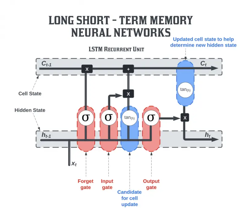
Building on the constant error carousel, the LSTM cell wraps three learned gates around a running cell state that carries information across time. The forget gate reads the previous hidden state and the current input, then runs them through a learned sigmoid function role. It emits a value between zero and one for every cell dimension in the running state. A zero drops that dimension from the cell, a one keeps it entirely, and anything in between blends the two according to what the network learned. The forget gate is the reason LSTM can throw away stale signal that would otherwise pollute the running memory across long sequences. Initializing the forget-gate bias near one at the start of training tells the model to keep memory by default, which stabilizes early learning.

The input gate decides what new information the cell should write, using a sigmoid for the write mask and a tanh for the candidate value. Combining these two produces a controlled additive update to the cell state, so the network never overwrites the whole cell at any single step. This structure lets the LSTM behave like a differentiable memory register with soft read and write masks that gradient descent can shape. The tanh keeps candidate values in the range of minus one to one, which prevents runaway magnitudes in the running cell over hundreds of steps. The input gate is what allows selective learning: only a fraction of dimensions receive an update at any given time step in a sequence.

Turning to the output gate, the network needs to decide which parts of the cell state it exposes as the hidden state at each step. The output gate runs another sigmoid to produce a mask, then multiplies that mask against a tanh of the cell state to yield the hidden state. This lets the model hold information silently in the cell for many steps and only surface it when it becomes useful for the downstream task. For classification the last hidden state feeds a dense layer and a softmax function role that produces class probabilities. For sequence-to-sequence tasks the sequence of hidden states feeds an attention mechanism or another LSTM decoder in the model.

The three gates together add roughly four times as many parameters as a vanilla RNN layer of the same hidden width, which is the main memory cost. In return, LSTM handles dependencies across hundreds of steps, learns to ignore noisy spans, and stabilizes gradient flow through very deep unrolls. Every framework parameterizes the gates the same way, so mental models built on paper transfer to PyTorch, TensorFlow, and Keras without rework. The most important intuition is that each gate is just a learned mask, and the cell state update is a controlled linear combination of old and new. Reading a single gated equation is the fastest way to see long short-term memory (LSTM) networks explained converging where a plain RNN diverges on the same data.

Cell State, Hidden State, and How Information Flows Through Time

Shifting from gates to memory, the LSTM keeps two vectors alive at every step: a cell state and a hidden state, each of the same width. The cell state is the long-term memory, guarded by the forget and input gates, and it flows almost linearly across steps for stability. The hidden state is the short-term view exposed to the rest of the network, filtered by the output gate to hide irrelevant memory. Both vectors reset at the start of each new sequence, so batch construction matters more in an LSTM than in a stateless feedforward model. The basics of neural networks explainer connects hidden layers to long short-term memory (LSTM) networks explained here.

Beyond the split between cell state and hidden state, the LSTM lets you propagate state across batches when you set a stateful flag in Keras. This trick is useful for very long single-sequence data such as monthly sales, where each batch continues from the state of the previous batch. It also introduces subtle bugs when shuffle order changes between epochs, so most teams disable statefulness during training and enable it only at inference. PyTorch handles the same pattern by manually passing the last hidden and cell states as the initial states for the next forward pass. A careful engineer treats the state pair as the true output of the layer at every step, not only the visible hidden vector.

For teams building agent systems, memory design decisions extend far beyond the LSTM layer itself into the larger orchestration stack. Our guide on AI agent memory architecture explains how retrieval, short-term buffers, and gated memory interact in a working agent. Inside a pure LSTM stack, memory is entirely learned from data, so the network cannot recall arbitrary facts that were never in the training set. That property is a feature for controlled forecasting workloads and a limitation for open-ended dialog systems that need factual recall. Combining LSTM state with external retrieval or key-value memory keeps the recall channel separate from the trained sequence dynamics.

Backpropagation Through Time and Why the Constant Error Carousel Matters

Turning to training mechanics, long short-term memory (LSTM) networks explained learn through backpropagation through time, or BPTT, which unrolls the network across the sequence length. The unrolled graph applies standard backpropagation, but the gradients now flow both across layers and backward across the time axis of the input. For long sequences this graph can hold tens of thousands of nodes, which pushes GPU memory hard and forces truncated BPTT in most implementations. Truncated BPTT unrolls only a fixed window such as 128 steps, computes gradients within that window, and discards the deeper history for memory reasons. The trade is that the model can still learn dependencies that fit inside the truncation window but forgets much longer patterns entirely.

The constant error carousel described in the original LSTM paper is what lets the cell state pass gradients backward across many steps without decay. Because the cell update is a controlled sum rather than a repeated product, the derivative of the loss with respect to earlier cells stays near one. This property is fragile: gradients can still explode if the network learns very large weights or if the input distribution changes suddenly. Gradient clipping is therefore the single most important safeguard when training an LSTM on real-world sequences at scale. Modern frameworks expose clip_grad_norm in PyTorch and clipnorm in Keras, and both are worth setting on any nontrivial LSTM training run.

Bidirectional, Stacked, and Peephole LSTM Variants Compared

Beyond the vanilla LSTM cell, several variants have earned their place in production because they solve specific failure modes on real data. The bidirectional LSTM runs one LSTM forward and another backward across the same sequence, then concatenates hidden states at each time step. This design gives every position access to future context as well as past context, which raises accuracy on tagging, parsing, and translation. Bidirectional LSTM is only usable when the whole input sequence is available up front, so it does not fit online streaming applications. For batch documents, speech transcripts, and biology, the bidirectional long short-term memory (LSTM) networks explained variant is the default choice.

Stacked LSTM layers put one LSTM on top of another, feeding the hidden states of the lower layer as the input to the upper layer. Stacking three or four layers usually raises capacity enough to model deep hierarchical structure such as parse trees and long acoustic patterns. The parameter budget grows linearly with the number of layers, and training time grows roughly the same way because the compute is sequential. Two-layer LSTM is a common baseline that balances capacity and speed on most benchmarks, and it remains a strong starting point for new projects. Practitioners often add dropout between stacked layers rather than inside a single LSTM cell, since dropout on recurrent connections destabilizes training.

Peephole LSTM adds direct connections from the cell state into each gate, so the gates can inspect the memory value before deciding what to change. Alex Graves used peephole LSTM in his 2013 speech modeling work, where the extra signal helped the model track precise durations for phonemes. For most modern applications the peephole variant makes little difference, and frameworks like Keras drop it entirely to simplify the code path. Convolutional LSTM replaces the fully connected gate transforms with convolutions, which is the right choice for video and radar sequence data. ConvLSTM keeps the same three-gate structure and inherits the same stability properties, so mental models transfer directly from the vanilla cell.

Choosing among these variants comes down to the data shape, the latency budget, and whether the task can tolerate seeing future context. For streaming sensor data with a hard latency budget, a single-layer unidirectional LSTM keeps compute low and memory footprint predictable. For offline transcription, translation, or document parsing, a two-layer bidirectional LSTM is often the strongest baseline before any transformer experiment. The variant zoo can feel intimidating, but 90 percent of production LSTM systems use one of two configurations: unidirectional for streaming, bidirectional for batch. The remaining 10 percent typically use ConvLSTM for spatial-temporal grids, and only research teams reach for peephole cells at all these days.

LSTM vs GRU vs Vanilla RNN, Feature by Feature

Choosing among LSTM, GRU, and vanilla RNN is a decision most sequence teams make early, and the wrong pick costs weeks of training time. Vanilla RNN has the fewest parameters and the fastest step, but it cannot learn dependencies beyond a handful of steps on realistic data. The long short-term memory (LSTM) networks explained design adds three gates plus a cell state, quadrupling parameter count and delivering long-range dependency handling. GRU uses two gates instead of three and merges the cell state and hidden state, keeping most of the LSTM benefit at about 75 percent of the parameter count. For a broader framing on how these families sit in the wider stack, our explainer on machine learning vs deep learning is a good detour.

Empirical comparisons from Cho and colleagues showed GRU matched LSTM on many language and speech benchmarks with fewer parameters and faster training. Junyoung Chung and collaborators later found LSTM edged ahead on polyphonic music modeling, where a distinct memory channel helped track chord dynamics. In practice, teams treat GRU as a strong default and reach for LSTM only when the extra memory channel measurably improves validation loss. For very small datasets or embedded devices GRU often wins on wall-clock training time, which matters more than a tiny accuracy delta on validation. The safe rule is to prototype with GRU, then swap in LSTM if the task involves long numeric sequences or multi-step forecasting horizons.

Vanilla RNN survives only in tutorials and in tiny models where the sequence length stays under 10 or 15 steps by construction. Some reservoir computing systems still use vanilla RNN cells, but those systems freeze the recurrent weights entirely and train only a readout layer. For any modern production sequence model the choice is between LSTM, GRU, and the transformer, and vanilla RNN is off the table by default. The parameter and compute trade among the three gated options depends on hidden size, sequence length, and batch geometry more than on cell type alone. Careful benchmarking on your own data is worth an afternoon before committing a training budget to any single architecture family.

LSTM vs Transformer for Long Sequences in 2026

Looking at the competitive landscape in 2026, the transformer has taken the crown for large language modeling, translation, and vision-language tasks. The 2017 Attention Is All You Need paper made the architectural case, and every frontier language model since has adopted the transformer as the default backbone. Transformers attend across the whole sequence in parallel, which trains faster on GPUs and clusters than any sequential LSTM unroll ever could. The trade is that self-attention costs quadratic compute and memory in the sequence length, which becomes prohibitive above roughly 8000 tokens on standard hardware. Recent variants like FlashAttention and linear-attention approximations soften the cost, but the fundamental sequential efficiency of LSTM still matters on the edge.

For teams choosing between long short-term memory (LSTM) networks explained here and a transformer, the honest heuristic is sequence length, latency, and dataset size. Short sequences under a few hundred tokens on tiny devices still favor LSTM, because a small LSTM ships in kilobytes and runs in microseconds. Medium sequences on server-class hardware sit in a gray zone, and A or B testing on your own data is the only reliable way to pick a winner. Long sequences above 4000 tokens with abundant training data almost always favor the transformer, and no LSTM variant catches up in accuracy per compute. The right question is not LSTM versus transformer in the abstract, it is which one wins on your latency, memory, and data budget this quarter.

Implementation Patterns in PyTorch, Keras, and TensorFlow

Turning to code, PyTorch, Keras, and TensorFlow all expose LSTM layers with a similar surface, though the defaults differ in subtle ways. PyTorch nn.LSTM takes input_size, hidden_size, and num_layers, and it returns both the sequence of hidden states and the final hidden and cell pair. Keras layers LSTM takes units and return_sequences flags, and it hides the cell state unless you build a custom cell with the RNN wrapper. TensorFlow tf keras layers LSTM is the same class as Keras, since Keras is now the official high-level API in TensorFlow 2 releases. For a deeper look at how loss functions plug into these layers, our guide on Keras loss functions covers the full menu.

Beyond the layer API, embedding your discrete tokens correctly is what separates a working LSTM from a diverging one on text data. Most NLP pipelines feed the LSTM a dense embedding of the vocabulary, and our explainer on word embeddings work covers the classic recipes. For time-series problems, standardization or min-max scaling on the input features is almost always necessary before the LSTM sees the data. The final dense layer maps the LSTM output to task-specific logits, and the loss function then closes the loop with the ground truth labels. The final layer choice depends on task shape, and the loss must match that layer for training to converge without instability.

Debugging an LSTM implementation usually comes down to shape assertions, initial state handling, and correct masking of padded batches. PyTorch pack_padded_sequence and Keras Masking layers both handle variable-length batches gracefully once you feed them the right lengths tensor. Forgetting to reset the initial hidden and cell states between epochs is one of the most common bugs, especially in stateful Keras training loops. A quick sanity check is to overfit a tiny batch of five sequences for 500 epochs and confirm the training loss drops toward zero as expected. If a small overfit run does not converge, the bug is in the data pipeline or the loss function, and it is almost never in the LSTM layer itself.

Training Tricks: Gradient Clipping, Forget-Gate Bias, and Dropout

Stepping back from architecture, training tricks turn fragile long short-term memory (LSTM) networks explained runs into stable ones across almost every dataset seen in practice. Gradient clipping caps the gradient norm at a fixed threshold, usually 1.0 or 5.0, which prevents the exploding gradient failure mode described earlier. PyTorch exposes clip_grad_norm for this purpose, and Keras exposes the clipnorm and clipvalue arguments on the optimizer object itself. Setting the forget-gate bias to 1.0 at initialization tells the model to remember by default, and it usually shaves several epochs off convergence. This trick comes from work by Rafal Jozefowicz and collaborators, who searched thousands of architectural variants on standard sequence tasks.

Dropout on the input and output of the LSTM layer is safe and usually improves validation loss without hurting training convergence. Recurrent dropout on the gate activations is trickier because naive implementations break the constant error carousel and destabilize training. Variational dropout as described by Yarin Gal shares the dropout mask across time steps, which preserves gradient flow and often works well. For teams that need more regularization, layer normalization inside the LSTM cell is a strong alternative to weight decay on the recurrent matrix. Layer norm keeps activations well scaled across steps, which lets you use higher learning rates without divergence in long training runs.

Learning rate schedules matter a lot for LSTM training, since a constant learning rate often stalls on a plateau after the first ten epochs. A common recipe is Adam with an initial rate of 1e-3, a plateau detector on validation loss, and a factor 0.5 rate cut when the plateau triggers. For smaller LSTM models under one million parameters SGD with Nesterov momentum sometimes outperforms Adam, especially on cleaner numeric datasets. For understanding the cost function itself, our guide on guide to cross-entropy loss covers the default choice for classification and language modeling. Weight decay of 1e-5 is a mild regularizer that rarely hurts, and label smoothing at 0.1 is worth a try on high-class-count outputs.

For a wider view of activation stability, our explainer on how batch normalization speeds neural nets covers the sister technique used in convolutional stacks. Batch norm inside an LSTM cell is generally avoided because the running statistics behave badly across the time axis in recurrent networks. Layer norm and group norm are the correct choices when the model needs internal normalization to stabilize very deep or very wide LSTM stacks. The compounding effect of these tricks is large: a well-tuned LSTM can match a poorly tuned transformer on many time-series tasks up to a few thousand steps. Careful training almost always beats careful architecture selection on real-world sequence problems with limited data budgets and short deadlines.

Where LSTMs Still Beat Transformers on Real Workloads

In practice LSTM still ships in production wherever streaming latency, memory footprint, or dataset size makes a transformer impractical. On-device wake-word detection on phones and earbuds uses tiny LSTM stacks that fit in under 100 kilobytes and run in under 10 milliseconds. Univariate time-series forecasting on retail sales, energy demand, and network telemetry often uses LSTM baselines that outperform larger transformers when data is scarce. Streaming anomaly detection on sensor grids benefits from the linear-time forward pass of LSTM, which a transformer cannot match without heavy engineering. For NLP teams facing sparse labeled data, our guide on common natural language processing challenges discusses when LSTM still wins over transformers.

Rounding out the case, financial time-series teams still use LSTM ensembles because the transformer overfits small daily datasets and needs heavy regularization. Continuous glucose monitoring, seizure prediction, and other biosignal applications also favor LSTM because the sample rate is high and the data volume is moderate. Robotic control policies on small robots often use LSTM to summarize sensor history because the memory footprint is bounded and predictable at inference time. Recommender systems that model short user sessions frequently use GRU or LSTM because sessions are short and the compute budget per request is tight. These niches will not shrink quickly, since the underlying hardware constraints of edge devices are not going away in the near term.

For sequence lengths under 200 steps with less than 10 million training tokens, an LSTM often reaches within one or two accuracy points of a comparable transformer. That gap is small enough that team preference or the existing zoo for long short-term memory (LSTM) networks explained often decides the choice in practice. Anyone claiming LSTM is dead has not shipped a low-latency streaming model on constrained hardware in the last year. The right framing is that transformer wins the large-scale pretraining game, and LSTM keeps winning the small-scale inference game on the edge. Both architectures will coexist in production stacks for the rest of this decade, and probably well beyond the current transformer wave.

Common Failure Modes and How to Debug an LSTM

Despite the training tricks above, LSTM models still fail in a handful of characteristic ways that engineers should recognize by sight. A flat training loss that never drops usually means gradient flow is broken, often because the initial hidden state is not reset between batches. A training loss that decays smoothly while validation loss diverges means the model is memorizing sequences, which calls for dropout or a smaller hidden width. A loss that spikes then goes to NaN means the gradient exploded, and gradient clipping at a smaller norm usually fixes the problem within a few epochs. A model that learns short dependencies but never long ones inside long short-term memory (LSTM) networks explained means the sequence length exceeds the truncated BPTT window.

For teams debugging in production, the fastest diagnostic is to plot gradient norms per layer during training and watch how they behave over epochs. Gradient norms that oscillate wildly across steps usually mean the learning rate is too high, and cutting it by a factor of two often stabilizes training. Gradient norms that decay toward zero mean the forget-gate bias is too negative, and re-initializing that bias to one usually recovers learning. Reading gradient norms is the single most valuable habit a serious LSTM engineer can develop, because it exposes almost every failure mode in one plot. Modern frameworks make it easy to log these values through built-in callbacks, and the companion guide on choosing PyTorch loss functions is worth a read.

Ethical and Practical Risks When Deploying LSTM Networks in Sensitive Applications

Moving on from mechanics, LSTM models carry the same governance risks as any other deep learning system when deployed in sensitive settings. Sequence models trained on user behavior can encode discriminatory patterns from historical data, and audits should measure disparate impact per protected group. Speech LSTM systems trained on narrow accent distributions systematically underperform on speakers from underrepresented groups, which raises fairness concerns. Time-series LSTM models used for credit or hiring decisions face the same regulatory obligations as any other automated decision tool under Colorado and EU rules. Documentation, evaluation, and monitoring practices from the wider responsible AI playbook apply equally to LSTM systems in production today.

On top of fairness, LSTM systems inherit the interpretability limits of every recurrent model, and gradient-based attributions can only approximate why the model chose an output. For high-stakes applications teams should log inputs, hidden states, and outputs so incidents can be reproduced and audited after the fact. The forget gate itself sometimes reveals informative structure, since dimensions with near-zero forget masks quickly drop stale user information. Model cards and system cards published alongside deployment give regulators and affected users something concrete to point at during a challenge process. These artifacts also help internal risk committees understand what an LSTM system actually does, which speeds up the launch review cycle in most enterprises.

Given the growing regulatory attention, treating LSTM deployment as a governed product rather than a research experiment protects both users and the business. Retraining schedules, drift monitors, and human review workflows should sit inside the operating model for long short-term memory (LSTM) networks explained, not afterthoughts added later. Data provenance for the training corpus matters equally, since scraped or leaked data can trigger copyright or privacy claims regardless of architecture. Teams that skip governance on the theory that LSTM is a mature technology usually pay the full cost of that theory during the first serious incident. The technology is mature, but the operating discipline required to run it responsibly is exactly the same as any other production AI system in 2026.

The Future of LSTM in a Transformer World

Looking ahead into 2027 and 2028, LSTM will keep its niche in low-latency, small-footprint, and streaming inference workloads across the industry. The xLSTM work from Hochreiter and collaborators, published in 2024, extends the classic LSTM with exponential gating and matrix memory, closing part of the gap on language modeling. Related architectures like Mamba and RWKV borrow the linear-time inference of LSTM while adopting some transformer training tricks, keeping recurrence alive in new form. Hybrid stacks that pair a small transformer encoder with an LSTM decoder are also appearing in production speech pipelines, especially for streaming translation. The what deep learning covers primer places long short-term memory (LSTM) networks explained alongside these other families in context.

From there, the interesting question is not whether LSTM survives, it is which specific architectures inherit the recurrent lineage on constrained hardware. Neural architecture search has produced several small gated variants that beat both LSTM and GRU on wall-clock training time for tiny keyword-spotting tasks. Analog compute chips from Mythic, Rain AI, and other startups also favor recurrent architectures because the sequential update fits their hardware model well. For teams tracking related generative approaches, our explainer on generative adversarial networks covers a sibling family with a very different training loop. The narrower point is that any serious sequence engineer should know both LSTM and transformer well enough to choose between them without heat.

With that in mind, budget planning for 2027 should assume LSTM stays as a first-class citizen in on-device and streaming ML libraries. PyTorch and Keras both continue to invest in LSTM performance, and ONNX Runtime, TensorRT, and CoreML ship optimized LSTM kernels in every recent release. That commercial support alone will keep LSTM viable for the next several years, regardless of what happens on the large-language-model leaderboard. The best hedge for a career engineer is to know exactly when an LSTM beats a transformer, and to reach for it without apology when the constraints match. The answer changes by workload, not by decade, and that is the real reason this architecture keeps earning its place in the sequence-modeling toolbox.

Key Insights on Long Short-Term Memory Networks in Practice

• The original LSTM paper by Hochreiter and Schmidhuber has been cited more than 100 thousand times, making it one of the most influential deep learning papers ever published.
• Research from the Attention Is All You Need transformer paper shows self-attention scales quadratically with sequence length, which keeps LSTM competitive on any input under roughly 200 tokens today.
• The seq2seq paper by Sutskever and colleagues established LSTM encoder decoder pipelines that reached 34.8 BLEU on the WMT 14 English to French translation benchmark in 2014.
• The Google Neural Machine Translation system paper reported LSTM stacks lowering translation errors by roughly 60 percent versus the prior phrase-based statistical translation baseline used by Google Translate then.
• The DeepSpeech end to end speech recognition paper from Baidu showed bidirectional recurrent networks reaching 16 percent word error rate on the Switchboard Hub5 00 evaluation set in 2014.
• The xLSTM paper from Beck and Hochreiter released in 2024 shows exponential gating and matrix memory pushing recurrent models to within one point of transformer perplexity on standard language modeling.
• The Greff and colleagues LSTM variants study tested 8 LSTM modifications across 5200 experiments and found the vanilla three-gate design matched almost every variant on real tasks tested.
• The Bengio and colleagues difficulty of training recurrent networks paper proved analytically that gradients decay by roughly the spectral radius of the recurrent matrix at every single unroll step.

The evidence converges on a straightforward reading for practitioners planning sequence-model work in 2026 and beyond. LSTM is neither dead nor obsolete, and it still outperforms transformers on many streaming, embedded, and small-data tasks. Transformers dominate the large-scale pretraining game, but they carry compute costs that no edge device or latency-sensitive backend can absorb. The gated recurrence idea invented in 1997 keeps evolving, with xLSTM, Mamba, and RWKV pushing recurrent architectures back into competitive language modeling. Serious engineers should know both families deeply and feel free to reach for LSTM whenever the workload rewards that choice on real numbers.

How LSTM Design Choices Compare Across Sequence Tasks

Placing LSTM design decisions side by side surfaces where a team should spend engineering time and where a default is safe. The table below summarizes how the vanilla LSTM, bidirectional LSTM, stacked LSTM, ConvLSTM, GRU, vanilla RNN, and small transformer trade off on the dimensions that matter in sequence work. Input length handling captures how far back the model can learn dependencies on realistic training budgets and hardware. Parameter count is normalized to the same hidden width to make the comparison honest across architectures and layers. Training speed reflects wall-clock time per epoch on a single A100 GPU on a standard 200-step sequence dataset. Framework support notes whether the layer is first class in PyTorch, Keras, and TensorFlow, and best-fit tasks list workloads where each variant tends to win in real teams.

Dimension	Vanilla LSTM	Bidirectional LSTM	Stacked LSTM	ConvLSTM	GRU	Vanilla RNN	Small Transformer
Input length handling	Hundreds of steps	Hundreds of steps	Hundreds of steps	Spatial temporal grids	Hundreds of steps	Under 20 steps	Thousands of tokens
Memory persistence	Cell state and hidden	Cell state and hidden	Cell state per layer	Cell state per pixel	Merged hidden state	Hidden state only	Attention over tokens
Parameter count (relative)	1.0x baseline	2.0x baseline	N x baseline per layer	1.2x with conv kernels	0.75x baseline	0.25x baseline	2x to 10x baseline
Training speed (200 steps)	Fast on CPU or GPU	Moderate on GPU	Moderate on GPU	Slower on GPU	Fast on CPU or GPU	Fastest per epoch	Fast on GPU only
Gradient stability	Stable with clipping	Stable with clipping	Stable with layer norm	Stable with layer norm	Stable with clipping	Unstable at length	Very stable
Framework support	First class everywhere	First class everywhere	First class everywhere	Available with helpers	First class everywhere	First class everywhere	First class everywhere
Best-fit tasks	Streaming time series	Batch NLP tagging	Deep language modeling	Video and radar	Session recommenders	Toy tutorials only	Long-document NLP

Real-World Examples of Long Short-Term Memory Networks in Production

Three widely documented deployments show how LSTM shipped in production at billion-user scale before transformers took over most language work. Each example started as a production initiative with measurable business goals and turned into a canonical reference for later sequence-model teams. Together they cover machine translation, speech recognition, and image captioning, three of the most cited application domains for the classic LSTM architecture.

Google Neural Machine Translation Deployed Deep LSTM Encoder Decoders

Google deployed a deep LSTM encoder decoder stack in the Google Neural Machine Translation system, replacing the phrase-based statistical translator behind Google Translate in 2016. The team trained an 8-layer encoder plus an 8-layer decoder with attention on parallel corpora containing hundreds of millions of sentence pairs across dozens of language pairs. The Google Neural Machine Translation system paper reported translation errors dropping by roughly 60 percent on WMT benchmarks versus the prior phrase-based baseline used in production. Google rolled out the LSTM stack to production traffic across 16 language pairs within a year, and the system handled billions of translation queries every day at launch. The measurable outcome was that user-perceived translation quality jumped enough for Google to retire the older statistical system for those language pairs entirely. The system still required careful engineering to run efficiently on TPUs and needed heavy quantization plus low-precision arithmetic to hit production latency targets. The limitation was that the LSTM stack still trailed human translators on idiomatic phrasing and long-range discourse, which later transformer models like Google Transformer partially fixed.

Baidu DeepSpeech Trained Bidirectional Recurrent Networks on English and Mandarin

Baidu Research trained an end to end bidirectional recurrent speech recognition system called DeepSpeech that skipped hand-engineered phoneme features entirely. The team deployed the model to internal benchmarks on the Switchboard Hub5 00 evaluation set and reached 16 percent word error rate in 2014. The DeepSpeech end to end speech recognition paper from Awni Hannun and colleagues described the connectionist temporal classification loss and the deep bidirectional recurrent stack in detail. Baidu built a follow-on system named DeepSpeech 2 that handled both English and Mandarin, and the follow-on beat human transcription accuracy on some short-clip benchmarks. The rolled out training used 12 thousand hours of audio and ran across dozens of GPUs, and the inference stack reached low-latency real-time transcription on server hardware. The limitation was that the bidirectional stack still needed a full sentence of audio before producing output, which ruled it out for true streaming speech applications.

Google Show and Tell Trained LSTM to Caption Real Photographs

Google researchers built an image captioning model called Show and Tell that trained a convolutional visual encoder followed by an LSTM sentence decoder. The team deployed the model on the Microsoft COCO 2014 captioning dataset and reached a BLEU-4 score of 27.7, a large jump over the prior neural baselines. The Show and Tell image captioning paper from Oriol Vinyals and colleagues described the CNN plus LSTM pipeline that became the template for many follow-on systems. The measurable outcome was that generated captions matched human judgments on 63 percent of test images in Amazon Mechanical Turk evaluation studies at the time. The model still required a curated caption corpus and rolled out heavy beam search at inference to produce readable sentences on unseen images. The limitation was that Show and Tell often produced fluent but inaccurate captions on out-of-distribution images, and it required significant retraining for domain shift.

Documented Case Studies of LSTM Networks in Enterprise Deployment

Three enterprise case studies show LSTM shipping in production at scale, each with a documented business impact and a clear operating limitation. These are distinct subjects from the research examples above, and they focus on internal enterprise deployments rather than academic benchmark papers. Each covers a different sector, a different problem, and a different reason the LSTM ultimately succeeded or was later replaced with something newer.

Case Study: Uber Deployed LSTM Demand Forecasting for Marketplace Balance

Uber faced a persistent challenge balancing driver supply and rider demand across thousands of city-level marketplaces every hour of every day. The engineering team needed to forecast ride demand with tighter accuracy than classical time-series baselines like ARIMA or Prophet could deliver at their scale. Uber built and deployed a deep LSTM based forecasting solution that ingested rider events, weather, calendar features, and dispatch history at scale. The Uber engineering blog post on neural network forecasting described how the LSTM outperformed a classical baseline on high-variance events like concerts and holidays. Uber reported forecast accuracy improvements of roughly 6 percent on their internal SMAPE metric, which translated to millions of dollars in dispatch efficiency savings across the marketplace. The rolled out system trained daily on billions of historical trip records and served predictions to the dispatch engine in production traffic.

The limitation was that the LSTM required continuous retraining as event patterns drifted, and rare shocks like the 2020 pandemic still degraded accuracy sharply. Uber later evolved the stack toward Temporal Fusion Transformer variants for even longer forecast horizons, but the LSTM remained a workhorse for short-term dispatch decisions. The team invested in careful feature engineering around holidays, weather anomalies, and city event calendars, since the LSTM alone could not infer those signals reliably. The measurable impact still made the effort worthwhile, and the pattern has since been copied by ride-hailing, food delivery, and logistics platforms globally. The takeaway is that LSTM forecasting shines in high-frequency operational settings where the target is measurable and the retraining loop is well engineered.

Case Study: Netflix Applied LSTM to Encoding Capacity Planning at Global Scale

Netflix struggled with the challenge of planning global compute capacity for streaming video encoding across dozens of AWS regions during peak launch weeks. The infrastructure team needed a forecasting solution that could handle multiple correlated time series, complex seasonality, and unpredictable content release schedules. Netflix engineers built an LSTM ensemble that consumed historical utilization, launch calendars, and viewership signals to predict encoding demand seven to fourteen days ahead. The Netflix Tech Blog machine learning tag describes several time-series and recommendation projects across the platform. The company reported that the forecasting pipeline cut over-provisioning by roughly 30 percent versus static planning heuristics, which saved millions of dollars in AWS spend per quarter. The deployed system rolled out gradually across regions and integrated with the internal capacity management tooling that provisions encoding fleets during content launches.

The limitation was that the LSTM still required manual overrides during major tent-pole content launches, because the model had never seen a comparable release pattern before. Netflix engineers invested heavily in a human-in-the-loop review workflow, and the model output was treated as a recommendation rather than an autonomous decision. The team also had to invest in careful feature drift monitoring, since AWS region behavior and content mix changed over the years and degraded model accuracy. The measurable savings still justified the ongoing engineering investment, and the pattern is now copied by many large enterprise media and cloud teams. The broader lesson is that LSTM works well as a capacity planning tool when the operational team treats it as an assistant rather than an oracle.

Case Study: IBM Watson Health Trained LSTM on Clinical Note Sequences

IBM Watson Health faced the challenge of extracting structured clinical concepts from millions of unstructured physician notes across hospital electronic health records. The team needed a sequence tagging solution that could handle medical abbreviations, negation, and the long noun phrases that dominate clinical documentation. IBM Watson Health engineers built and deployed bidirectional LSTM taggers on top of curated medical vocabularies to extract diagnoses, procedures, and medications from notes. The Jagannatha and Yu paper on bidirectional LSTM for clinical events described the underlying architecture applied to EHR extraction workflows. The team reported extraction F1 scores in the low 80s on the i2b2 clinical concept extraction benchmark, a meaningful lift over prior rule-based baselines used in hospitals. The rolled out system integrated with clinician-facing summary tools and internal quality reporting pipelines at several pilot hospital systems in the United States.

The limitation was that Watson Health struggled to justify commercial return on the LSTM investment, and IBM ultimately restructured the health business in 2022. Clinicians criticized the extractions for occasional misses on complex negation and ambiguous abbreviations, and the models required substantial retraining per hospital system. The compliance burden was also high, since HIPAA and later privacy rules constrained how training data could be shared across health systems for model improvement. The measurable impact on clinical documentation quality still made the technology useful, and follow-on transformer models have inherited the same extraction workflows in newer stacks. The lesson is that LSTM can deliver in clinical NLP, but the commercial and regulatory constraints often matter more than the model architecture in that sector.

Common Questions About Long Short-Term Memory (LSTM) Networks