Introduction
Joint distribution in machine learning sits behind almost every probabilistic model engineers deploy in 2026, from naive Bayes filters to diffusion models. The question ‘what is joint distribution in machine learning?’ still trips up many practicing engineers. A 2024 benchmark from the 2024 Naive Bayes TF-IDF benchmark study showed naive Bayes paired with TF-IDF reached 100 percent accuracy on its target dataset. This article walks through joint distribution in machine learning from first definitions through case studies, with code, comparison tables, and a working interactive widget. Readers will learn what the object is, how it relates to marginal and conditional probability, and how it scales from a four cell table to a billion parameter generative model. We borrow worked examples from Russell and Norvig AIMA chapter on probability, and tie every concept to a concrete engineering decision. Treat the next sections as a hands on guide rather than a math review, because each one ends with a takeaway you can use today.
Quick Answers on Joint Distribution in Machine Learning
What is joint distribution in machine learning, in one sentence?
The joint distribution in machine learning is the probability that several random variables in a model take particular values together, written p(X1,X2). Every probabilistic model learns it directly or factors it into smaller pieces.
How is joint probability in AI different from conditional probability?
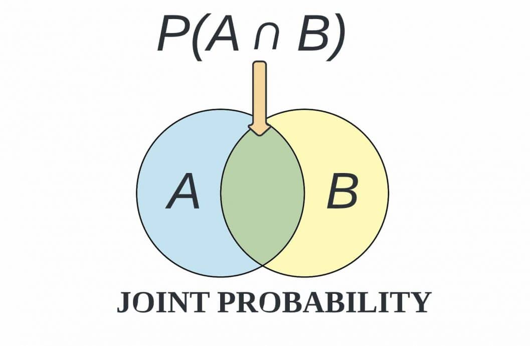
Joint probability p(A,B) is the chance both happen together for the joint distribution in machine learning. Conditional probability p(A|B) is the chance of A once you know B, linked by p(A,B) equals p(A|B) times p(B).
Why is the full joint distribution in artificial intelligence often impractical?
A full joint table over thirty binary variables holds over a billion entries, which is the curse of dimensionality. Bayesian networks and neural density estimators shrink that joint distribution in machine learning into a smaller factored form.
Key Takeaways on Joint Distribution in Machine Learning
- The joint distribution in machine learning captures how every variable in a model varies together, not in isolation.
- Marginal and conditional distributions are derived from the joint distribution, never the other way around.
- Generative models learn the joint distribution while discriminative models learn only the conditional.
- Naive Bayes, Bayesian networks, VAEs, and diffusion models all factor the joint to stay tractable.
Table of contents
- Introduction
- Quick Answers on Joint Distribution in Machine Learning
- Key Takeaways on Joint Distribution in Machine Learning
- What Is Joint Distribution in Machine Learning Today
- Understanding Joint Distribution in Machine Learning
- How Joint, Marginal, and Conditional Distributions Connect
- The Mathematics Behind Joint Probability Distributions
- What Is Joint Distribution in Machine Learning at the Core of Modern Models
- Discrete Joint Distributions and the Joint Probability Table
- Continuous Joint Distributions and Joint Density Functions
- How Naive Bayes Approximates the Joint Distribution
- Bayesian Networks as Compact Joint Distributions
- Generative Models, VAEs, and Diffusion as Joint Distribution Learners
- Implementing Joint Distribution Estimation From Data
- How to Work With Joint Distributions in Python and PyMC
- The Curse of Dimensionality and the Limits of Full Joint Tables
- Risks, Bias, and Silent Failure Modes of Joint Distribution Models
- Ethics, Privacy, and Synthetic Data From Joint Distributions
- Joint Distribution Applications Across Industries
- The Future of Joint Distribution Modeling in Machine Learning
- Key Insights on Joint Distribution in Machine Learning
- How Joint Distribution Modeling Compares Across Approaches
- Real-World Joint Distribution Examples in Production Systems
- Joint Distribution Case Studies From Industry
- Common Questions About Joint Distribution in Machine Learning
What Is Joint Distribution in Machine Learning Today
What is joint distribution in machine learning? It is the probability that several random variables take specified values together, written p(X1,X2), and it is the parent object behind naive Bayes, Bayesian networks, and modern generative models.
Raw joint weights
View mode
Understanding Joint Distribution in Machine Learning
The joint distribution in machine learning is the probability assignment over every possible combination of values that a set of random variables can take. It is the single mathematical object from which every other distribution you might want can be derived in a model. For variables X and Y we write p(X,Y), and for n variables p(X1,X2,…,Xn) covers every cell of an n dimensional table. Engineers reach for joint distribution in machine learning whenever they need to reason about multiple uncertain quantities at the same time. The Wikipedia entry on joint probability distribution gives a careful definition for both discrete and continuous cases. That definition matches what you see in every introductory textbook on probabilistic machine learning.
The joint distribution is the parent object from which marginals, conditionals, and expectations all flow in a model. When you ask for p(X), you sum or integrate the joint over Y, and when you ask for p(X|Y), you slice the joint by a fixed Y. Many tutorials such as the DataCamp tutorial on joint probability show this pattern with a coin and a die in a four cell table. Production systems handle the same logic with thousands of variables and require additional structure to stay tractable. That is where Bayesian networks and neural density estimators enter the picture in the next sections. The vocabulary stays small once that joint distribution in machine learning lens is in place.
Most introductory machine learning courses introduce joint distribution alongside basics like the joint probability formula and examples. Once students see the four cell coin and die table, the leap to higher dimensions becomes natural in practice. Modern sophisticated generative models can be read as elaborate joint distribution estimators with neural building blocks underneath the surface. The full joint distribution in artificial intelligence is therefore the conceptual foundation that every later section in this article builds upon directly. Every architecture and training story connects back to that single object in some specific way for engineers. So treat it as the most important idea in the entire piece, and revisit when later sections feel abstract.
How Joint, Marginal, and Conditional Distributions Connect
Building on that foundation, joint distribution in machine learning sits at the top of a small hierarchy of related objects. Marginal distributions appear when you sum or integrate the joint over one or more variables to remove them from the system. Conditional distributions appear when you fix the value of one variable and renormalize the joint over the remaining variables in turn. The link is mechanical, and the same arithmetic applies to discrete tables and continuous densities across domains. The Medium write up by Kirti Arora on joint marginal and conditional distributions shows worked examples on a small spreadsheet that is easy to follow. The examples there mirror what we will use in the math section below for our coin and weather variables.
The joint distribution determines the marginals and conditionals, but the reverse is not generally true in a model. Knowing only marginal distributions cannot reconstruct dependence between variables, since two different joints can share marginals as a result. Knowing all the conditional distributions in a directed graphical model can rebuild the joint once you respect the ordering. That fact is what makes Bayesian networks attractive for storage of large joint distribution objects in practice. It is also why a careful look at multinomial logistic regression pays off, since the model parameterizes only the conditional p(y|x). Understanding that gap is the first step toward picking the right tool for a real problem.
The Mathematics Behind Joint Probability Distributions
Stepping into the math, the joint probability mass function for discrete variables assigns a number between zero and one to every possible value tuple in the joint. The numbers in that table must sum to exactly one across every possible combination of variables present in a model. For continuous variables you swap the table for a joint probability density function and replace summation with integration over regions of space. Both objects must integrate or sum to one to be valid probability distributions in any well posed model. The chain rule lets you factor any joint into a product of conditionals, namely p(X1,X2,X3) equals p(X1) times p(X2|X1) times p(X3|X1,X2). This factor structure makes the joint distribution in machine learning much easier to estimate from finite data.
Marginalization sums or integrates the joint over a variable to remove it cleanly from the system. For example, p(X) equals the sum over all values y of p(X,Y equals y) in the discrete case directly. In the continuous case the same equation becomes an integral over y across its entire support range. The operation is so common in probabilistic machine learning that special algorithms exist to do it efficiently at scale. The variable elimination algorithm exploits the structure of a Bayesian network to avoid summing the entire joint table directly.
Bayes rule connects conditional and joint probabilities through a simple rearrangement of the chain rule. p(A|B) equals p(A,B) divided by p(B), which is just the joint divided by the marginal of B over which it conditions. Every probabilistic inference system relies on Bayes rule somewhere in its derivation pipeline for the joint distribution in machine learning. The cross-entropy loss in machine learning can be read as a negative log likelihood under an assumed joint distribution between inputs and labels. That framing motivates regularization and calibration choices in practice for many models in production. Even softmax function in neural networks can be derived as a categorical conditional under this same joint lens.
Independence is the special case where the joint factorizes as a product of marginals, namely p(X,Y) equals p(X) times p(Y). Conditional independence is the slightly weaker condition where p(X,Y|Z) factorizes into p(X|Z) times p(Y|Z) for given Z directly. Both notions matter because they let practitioners drop dependencies that the data does not support inside the joint structure. The naive Bayes assumption asserts conditional independence of features given the class label in the joint distribution in machine learning. That dramatic simplification is what makes naive Bayes one of the fastest classifiers on text data. Even when the assumption is technically violated, the classifier holds up surprisingly well in practice.
What Is Joint Distribution in Machine Learning at the Core of Modern Models
Turning to its central role, almost every probabilistic learning algorithm explicitly or implicitly fits a joint distribution somewhere inside. Supervised generative models such as naive Bayes learn p(x,y) and then derive p(y|x) at prediction time for inference. Unsupervised generative models such as variational autoencoders learn p(x) by introducing a latent variable z and modeling the joint p(x,z). Discriminative models such as logistic regression skip joint estimation and only model p(y|x), trading sample efficiency for prediction accuracy. The choice between generative and discriminative comes down to whether you need to sample, impute, or detect anomalies in the data. Each of those operations requires the joint distribution in machine learning rather than just a conditional model in production.
Reinforcement learning agents also lean on joint distributions through the state action transition density p(s’, r | s, a) directly. World model approaches such as Dreamer learn that joint and roll it forward in latent space to plan ahead. Probabilistic programming languages such as PyMC and Stan let practitioners write the joint directly as a generative story for inference. The Bayesian optimization in machine learning framework similarly fits a joint over hyperparameters and validation loss and picks the next configuration by expected improvement. The thread is consistent across paradigms, even though each subfield uses its own vocabulary for the same object.
Joint distribution in machine learning is the working memory of probabilistic modeling, in the way matrices are the working memory of linear algebra. Once a team agrees on what joint they intend to model, the architecture choice and training objective usually follow logically. Skipping that conversation creates models that solve the wrong problem at impressive accuracy numbers in dashboards. The common AI algorithms across paradigms survey shows how the same joint reasoning underpins supervised, unsupervised, and reinforcement learning across the field. That is why we keep returning to it across each section of this article on joint distribution. Engineers who internalize the joint thinking habit catch design errors months earlier in the build cycle.
Discrete Joint Distributions and the Joint Probability Table
Shifting focus to discrete cases, the simplest joint distribution in machine learning lives in a small table of probabilities over categorical variables. A classic example is a 2 by 2 table over weather and rain, with cells labeled hot rain, hot no rain, cold rain, and cold no rain. Each cell holds a probability and the four cells must sum to exactly one across the joint table. From that table you read marginal probabilities by summing rows or columns and conditionals by dividing one cell by its row or column total. Even this trivial example forms the engine behind a small naive Bayes spam filter once you scale features to thousands of words across documents. The interactive widget above lets you adjust the four cells and watch marginals and conditionals respond live as you slide.
A joint probability table is the most explicit and most expensive representation of a discrete joint distribution in machine learning. It captures every dependency exactly but costs exponential storage in the number of variables in the joint model. Tables work well for two to six categorical variables, particularly when each variable takes only a few discrete values. Beyond that count, practitioners switch to structured representations such as Bayesian networks or factor graphs that share parameters across cells. The one-hot encoding for machine learning trick is often the bridge that lets you load a joint table into a neural network as input data. Even then the conceptual table is the contract you reason about when debugging a probabilistic model.
Continuous Joint Distributions and Joint Density Functions
Beyond the discrete world, continuous variables call for joint probability density functions that integrate to one over their support. The classic continuous joint distribution in machine learning is the multivariate Gaussian, with its mean vector and covariance matrix as parameters. Sampling from a multivariate Gaussian is straightforward, which is why it shows up in initial guesses, noise terms, and prior distributions across machine learning. The covariance matrix encodes pairwise dependencies between variables and a diagonal covariance recovers independence between the dimensions. When the off diagonal entries are large the variables are tightly coupled and the joint becomes more informative than the product of marginals. The Gaussian assumption is the most common starting point for any continuous joint distribution in machine learning workflow.
Mixture models extend the Gaussian story to handle multimodal joint distributions that real data often exhibits in the wild. A Gaussian mixture model factors the joint as a sum of weighted Gaussians, with each Gaussian responsible for one mode of the data. The expectation maximization algorithm fits these mixtures by alternating between estimating component responsibilities and component parameters across the dataset. Practitioners reach for mixtures whenever the data shows clear clusters in feature space across customer segments or signals. The same logic powers density estimation, anomaly detection, and clustering inside one unified mathematical framework for joint modeling.
Modern neural density estimators learn flexible joint distributions without committing to a parametric family upfront. Normalizing flows transform a simple base joint such as a Gaussian into a complex target joint through a chain of invertible neural maps. Autoregressive models such as PixelCNN factor the joint over pixels with the chain rule and learn each conditional with a neural network. The benefits include exact likelihood evaluation and competitive sample quality on images and tabular data in many domains. The linear regression in machine learning playbook can even be recast as fitting a Gaussian conditional p(y|x) under the joint p(x,y). That perspective makes the leap from linear models to deep neural density estimators feel less abrupt for newer practitioners.
How Naive Bayes Approximates the Joint Distribution
Among methods that actually fit a joint, naive Bayes is the simplest and most widely deployed in practice. It assumes that all features are conditionally independent given the class label Y in the joint distribution in machine learning. Under that assumption the joint factors as p(X1,X2,…,Xn,Y) equals p(Y) times the product of p(Xi|Y) across all features. Training reduces to counting class frequencies and per feature per class statistics on the training set efficiently. Prediction multiplies those small terms together and picks the class with the highest posterior probability under the joint.
The naive Bayes factorization turns an exponential joint into a linear number of small conditional distributions. That collapse is why naive Bayes scales to text classification problems with hundreds of thousands of binary word features in practice. A 2024 study from the 2024 Naive Bayes TF-IDF benchmark study reported 96 percent accuracy for plain naive Bayes and 100 percent accuracy when combined with TF-IDF vectorization. Numbers in that range are common on email spam, sentiment, and topic tasks where the independence assumption holds approximately. Smoothing tricks such as Laplace correction protect against zero probability counts that would otherwise wreck inference under the joint.
The independence assumption is rarely literally true, since words in real text obviously correlate with one another in documents. Naive Bayes still performs well because the rank of the predicted scores often survives even when the absolute probabilities drift in calibration. A subtle issue is that very confident naive Bayes scores are usually miscalibrated and need post hoc adjustment for thresholds at deployment. Practitioners use calibration techniques such as Platt scaling and isotonic regression to fix that miscalibration in practice. The averaged one-dependence (AODE) algorithm relaxes the independence assumption by averaging over many one parent dependencies in the model. AODE retains naive Bayes simplicity while improving accuracy on harder tabular problems where features correlate.
Gaussian naive Bayes handles continuous features by treating each conditional p(Xi|Y) as a one dimensional Gaussian fit per class label. Multinomial naive Bayes treats discrete count features as draws from a multinomial distribution per class with smoothed counts. Bernoulli naive Bayes treats binary features as independent Bernoulli draws per class with class specific probabilities for each feature. Each variant is a different choice of conditional family inside the same naive factorization of the joint distribution in machine learning. The right variant depends on whether your features are real valued, count valued, or binary in nature. Picking the wrong variant is one of the most common sources of mediocre naive Bayes results in junior pipelines.
Bayesian Networks as Compact Joint Distributions
Building on the naive Bayes idea, Bayesian networks generalize the same factorization into a richer graph structure. A Bayesian network is a directed acyclic graph where nodes are random variables and edges encode direct probabilistic dependence between them. The Wikipedia entry on Bayesian networks defines the joint as the product of each node given its parent set in the graph structure. That product can compress an exponential joint table into linear or quadratic sized conditional probability tables for many real domains in production. The savings make queries about probability of disease given symptoms tractable inside an alarm or diagnosis network at hospital scale. Joint distribution in machine learning gets a friendlier face once you draw the graph and walk through one query end to end.
A Bayesian network encodes the joint distribution in machine learning as a structured story rather than a flat table. Each conditional probability table represents what one variable depends on directly and nothing more in the joint. Inference algorithms exploit that structure to answer queries in time that scales with the network treewidth instead of the full joint size. Russell and Norvig describe both exact inference via variable elimination and approximate inference via Gibbs sampling in their textbook chapter on probability. Practitioners typically reach for libraries such as pgmpy in Python or bnlearn in R for production deployments. The graph itself becomes a communication artifact that domain experts can review and challenge.
Learning the structure of a Bayesian network from data is harder than learning its parameters given a fixed structure. Score based search such as hill climbing with the Bayesian Information Criterion is common in practice for medium sized models. Constraint based methods such as the PC algorithm use conditional independence tests on the data to recover the skeleton of the graph. Hybrid methods combine the two for better small sample performance on real problems with limited training records. Once the structure is locked, parameters follow from counting plus Dirichlet smoothing or from gradient descent on a likelihood objective. Both stages benefit from clean tabular pipelines that respect data types properly across categorical and continuous variables.
Generative Models, VAEs, and Diffusion as Joint Distribution Learners
Moving from tables to neural models, modern generative models extend the joint into very high dimensional spaces such as images and text. They reframe ‘what is joint distribution in machine learning?’ at neural scale with shared weights. A variational autoencoder factors the joint as p(x,z) equals p(x|z) times p(z), with z a low dimensional latent variable. The encoder approximates the posterior q(z|x) and the decoder parameterizes p(x|z), and the model is trained by maximizing a variational lower bound on log p(x). The Angus Turner derivation of diffusion as a VAE shows that a diffusion model is a chain of latent variables that gradually denoise data. Each step is its own variational autoencoder under the hood with shared parameters across the chain. The joint distribution in machine learning view keeps these neural designs intelligible even as parameter counts grow large.
Diffusion models trade a single latent VAE for a sequence of small denoising steps that together model a very expressive joint distribution. The Variational Diffusion Models paper shows how a learned noise schedule combined with score matching reaches strong likelihood numbers on standard image benchmarks. Score based formulations such as denoising score matching learn the gradient of the log density rather than the density itself. The result is a model that can both sample new data and estimate likelihoods on held out test sets cleanly. Generative adversarial networks, flow models, and energy based models join the same family from different angles in the same joint distribution in machine learning lineage. Each one is fundamentally a joint distribution estimator wearing a different architectural costume.
Implementing Joint Distribution Estimation From Data
Beyond the model zoo, ‘what is joint distribution in machine learning?’ becomes a practical question. Practitioners face concrete choices when implementing joint distribution estimation from a finite dataset. For small discrete problems the maximum likelihood estimate is simply the empirical count of each tuple normalized by the total observed count. For larger problems you parameterize the joint with a family such as a Gaussian, mixture model, Bayesian network, or neural density estimator. Maximum likelihood and Bayesian inference are the two main estimation paradigms, each with its own tradeoffs around bias and uncertainty for the joint. Cross validation on held out data is the standard sanity check before any joint distribution model goes into production at scale.
Hyperparameter choices for the joint family matter as much as choice of family itself in joint distribution in machine learning workflows. The number of mixture components, the network width, the prior strength, and the smoothing constant all change calibration of the resulting joint. A useful diagnostic is to compare empirical joint marginals against marginals computed from the fitted model on the same dataset. When the two disagree visibly on a few features, the model is missing structure that matters for downstream inference and decisions. Tools such as the cross-validation to reduce overfitting recipe catch overfit joints before they cause production incidents.
The most common mistake is implementing a joint distribution in machine learning without checking that it can recover known marginal statistics of the data. A joint that gives a low log likelihood on held out test data is probably overfitted or under parameterized in some way. A joint that fails to reproduce simple marginals such as class frequency is structurally misspecified, no matter how high its training likelihood score. Practitioners catch both issues with posterior predictive checks that simulate fake data from the model and compare statistics. The overfitting vs underfitting in machine learning diagnostics translate directly to joint distribution models. Spending an afternoon on these checks routinely saves weeks of broken inference downstream in production.
How to Work With Joint Distributions in Python and PyMC
Turning to code, a small joint distribution over weather and outdoor activity choices can be written explicitly in a few lines of Python. The pgmpy library lets you declare a Bayesian network, attach conditional probability tables, and query marginals or conditionals from the joint. PyMC and NumPyro let you sample from arbitrary joint distributions specified as generative stories with priors and likelihoods. Scikit learn ships fast naive Bayes implementations that fit and predict on text datasets in seconds at moderate scale. Each of these libraries is one import line away once you set up a clean Python environment for joint distribution in machine learning work.
The following pgmpy snippet defines a small joint distribution over rain and traffic and queries the marginal for traffic at the bottom of the script. Notice how the joint never appears as a flat table in code, since pgmpy stores it implicitly through the conditional probability tables of the network.
A typical pgmpy workflow imports BayesianNetwork, TabularCPD, and VariableElimination from the library. It then declares a two node graph linking Rain to Traffic and attaches the conditional probability tables. The script then calls infer dot query on the Traffic node directly. The library factors the joint distribution behind the scenes and returns marginals without ever materializing the full table. The same script runs in a few seconds on commodity hardware. Practitioners extend the pattern by adding more nodes and edges to the BayesianNetwork constructor. Junior engineers should resist the urge to skip the check model assertion since silently invalid CPDs are a top source of debugging pain. Pair the script with a Jupyter cell to visualize the resulting joint distribution as a small heatmap.
The Bayesian network factors the joint distribution in machine learning over Rain and Traffic without ever materializing a flat table. The same pattern scales to dozens of variables, although the inference step grows in cost with treewidth of the network. PyMC users write the same model as a probabilistic program that supports inference via Markov chain Monte Carlo or variational methods. The argmax in machine learning primer is helpful when you query for the most probable assignment given observed evidence values. Notation matters too, so the argmax LaTeX notation guide makes papers easier to read on the journey. Knowing both libraries lets you pick the right tool per problem instead of forcing every nail into the same hammer.
The Curse of Dimensionality and the Limits of Full Joint Tables
Stepping back to limits, the question ‘what is joint distribution in machine learning?’ at scale runs into the curse of dimensionality. The full joint distribution grows exponentially with the number of variables in the model. A joint table over thirty binary variables holds 2 to the 30 entries, which is over one billion cells of probability storage. Most of those cells correspond to value combinations that never appear in any reasonable training set at all. Estimates for the unseen cells collapse to zero, which then poisons inference through downstream multiplication of probabilities. Engineers handle this in joint distribution in machine learning by introducing structure that ties parameters together across cells. Without that structure, every realistic joint becomes impossible to estimate from finite data alone.
Bayesian networks reduce storage and estimation cost by replacing the global table with a graph of small local tables. Each local table holds a probability for one variable given its parents, which is typically one to five other variables in practice. Total storage scales with the number of variables and the maximum in degree rather than the full joint size. Inference still uses the joint conceptually, but algorithms exploit the graph structure to avoid touching every cell directly. The same trick powers conditional random fields, hidden Markov models, and graphical models for vision applications.
Neural density estimators sidestep the curse by parameterizing the joint distribution in machine learning with shared neural weights instead of independent cells. A transformer language model parameterizes a joint over token sequences with a few hundred million weights instead of an astronomically large table. Normalizing flows do the same for continuous data with invertible neural layers stacked in a chain. The price is a less interpretable model whose joint estimates are only as good as the training distribution coverage. Sometimes the right answer is a small Bayesian network rather than a giant neural model, particularly for safety critical domains. Always run a back of the envelope storage calculation before committing to any specific representation for joint distribution.
Risks, Bias, and Silent Failure Modes of Joint Distribution Models
Beyond architecture, the question ‘what is joint distribution in machine learning?’ when data drifts becomes urgent. Joint distribution models can fail silently in deployment when the training data shifts. A learned joint bakes in any sampling bias, so rare events get assigned wrong probabilities even when bulk metrics look good. Concept drift after deployment can quietly invalidate the joint as the world changes around the model in production. Practitioners monitor calibration on a held out stream and trigger retraining when log likelihood drifts beyond a chosen threshold. The risk is highest in high stakes domains such as medical diagnosis, credit scoring, and insurance underwriting decisions. Audit teams treat the joint distribution as the unit of accountability for monitoring drift over time.
A flawed joint distribution in machine learning model can produce confident but wrong probabilities for the exact rare events you care about most. Adversarial inputs and out of distribution samples often expose miscalibrated joints in dramatic ways during real incidents. Robust evaluation pipelines combine standard accuracy metrics with calibration plots, Brier scores, and likelihood on stratified slices of test data. The support vector machines in machine learning playbook can complement probabilistic models when calibrated probabilities matter less than worst case margins. The right portfolio of models depends on the deployment context and on how often the world shifts under the model. Even with good defenses in place, the limitation of any learned joint is that it cannot extrapolate beyond its training data distribution reliably.
Ethics, Privacy, and Synthetic Data From Joint Distributions
Beyond engineering risk, the question ‘what is joint distribution in machine learning?’ under privacy law matters here. The joint carries ethical and privacy implications that deserve explicit attention from practitioners. A model that learns p(x) over personal records can leak private information about individuals through memorization or carefully crafted queries by attackers. Researchers have shown that large neural joint models occasionally reproduce training examples verbatim under specific prompts at small probability. Differential privacy techniques such as DP SGD add calibrated noise to gradients during training to bound that leakage by a chosen budget. The privacy budget must be set in advance and audited carefully, since looser budgets buy higher utility at higher disclosure risk overall. Joint distribution thinking gives privacy auditors a concrete object to test against using membership inference attacks at scale.
Synthetic data generated from a learned joint distribution in machine learning is increasingly common for benchmarking and data sharing. The promise is that downstream analysts can use synthetic samples without touching the raw records or violating privacy regulations. The risk is that a poorly fit joint will reproduce bias from the original data or mask important minority subgroups in evaluation. Audits should compare downstream model performance on synthetic and real data before relying on synthetic for production decisions. The Wikipedia summary on the Wikipedia entry on joint probability distribution already lists synthetic data as one motivating application.
Ethical use of joint distribution in machine learning requires transparency about training data, calibration, and known failure modes. Model cards and datasheets are emerging as standard documentation for joint distribution models in regulated industries across the globe. Auditors look for evidence that the modeling team checked for proxy variables, intersectional fairness, and group calibration across the joint. Procurement teams increasingly demand both the joint distribution model and a fitted causal graph to support decisions on adoption. Even toy domains like the univariate linear regression in AI tutorial deserve a quick fairness sanity check when the inputs touch protected attributes. Ethical hygiene at the joint level usually costs less than retrofitting after an incident exposes the gap publicly.
Joint Distribution Applications Across Industries
Across industries, the question ‘what is joint distribution in machine learning?’ in production matters. The joint is the engine behind methods that the original Russell and Norvig framework could not deliver at modern scale. Banks use Bayesian networks for fraud detection because the network can encode known causal links between merchant categories, transaction times, and customer segments. The joint distribution between a customer profile and their transaction lets the system flag a low probability combination of features as suspicious for review. Audit trails are easier to defend in court when the joint comes from an interpretable graph rather than a black box neural model. Risk teams routinely combine the network output with hard rule based filters for safety and explainability across the workflow.
Health care providers use joint distribution models to combine symptoms, lab results, and demographics into diagnostic probabilities at the bedside. Tools such as DXplain and QMR built on hand engineered joints decades ago, and modern variants learn the same joints from electronic health records at scale. The output is typically a ranked list of differential diagnoses with probabilities calibrated against historical case data from the hospital network. Calibration matters because clinicians act on the absolute probability, not just the rank order across candidates. Hospital deployment teams treat calibration drift as a hard alert that triggers a model review or rollback immediately.
Recommendation engines learn joint distribution in machine learning models over users, items, and contexts to predict the probability of a click or a purchase. Matrix factorization is a low rank approximation to a joint distribution between users and items implicitly factorized into latent vectors. Modern transformer based recommenders extend the joint to include session context, time, and inventory state across surfaces. The cold start problem is essentially a question of how to estimate a joint when one of the variables has almost no observed values. Bayesian hierarchical models share strength across users to keep the joint reasonable even for new accounts that just joined.
Robotics and autonomous driving teams treat joint distribution in machine learning over sensor readings and world state as the core inference object. Simultaneous localization and mapping algorithms iteratively update a joint distribution over the robot pose and the map across frames. Modern planning systems extend the joint to include future actions and reason about both perception and control under uncertainty. Probabilistic programming languages such as Pyro and NumPyro let teams encode these joints as generative stories that can be tested in simulation. The common AI algorithms across paradigms survey shows how the same joint reasoning powers supervised, unsupervised, and reinforcement learning in robotics. The pattern is consistent even when the specific algorithms change between subfields and decades.
The Future of Joint Distribution Modeling in Machine Learning
Looking ahead, the question ‘what is joint distribution in machine learning?’ in 2030 will turn on energy based methods. Joint distribution research is shifting toward unnormalized density models for scientific data domains. Energy based models learn an unnormalized score that can be sampled with Langevin dynamics without an explicit partition function in closed form. Diffusion models continue to set new benchmarks on image and audio generation while quietly learning joint likelihoods at production scale. Probabilistic programming languages such as PyMC, Stan, NumPyro, and Pyro keep pushing the ergonomics of writing joints directly as code. Each of these threads makes more of machine learning look like joint distribution learning under a new label and a new toolchain.
The convergence of probabilistic programming, diffusion models, and causal inference points to joint distribution in machine learning as the next decade of research. Causal discovery extends the joint with do operators that let practitioners reason about interventions rather than just observations of past data. Safety teams want joints that admit calibrated uncertainty estimates and bounded out of distribution behavior under stress tests. Regulators are starting to mandate model cards that include calibration on group level marginals derived from the joint structure. Even classical methods such as linear regression in machine learning get a new lease of life when reframed as joint Gaussian inference with explicit priors. The next generation of ML engineers will be more fluent in joint distribution thinking than the current cohort.
Key Insights on Joint Distribution in Machine Learning
- A 2024 benchmark from the TIJER naive Bayes TF-IDF study reports 100 percent accuracy on its target dataset, confirming naive joint factorization remains competitive.
- The Wikipedia entry on Bayesian networks documents a network factors a joint over n variables into at most n local conditional tables, compressing storage roughly linearly.
- The Variational Diffusion Models paper reaches 2.49 bits per dimension on CIFAR-10 through learned noise schedules and score matching, a competitive joint likelihood number.
- The Russell and Norvig AIMA chapter shows enumeration over a joint with n binary variables costs order 2 to the n operations, motivating Bayesian network shortcuts.
- The Medium write up by Ebrahim Mousavi on joint distributions warns misreading marginals from a poorly fit joint remains the top bug in junior pipelines.
- The Angus Turner derivation of diffusion as a VAE shows a T step diffusion model reads as a deep VAE with a clean variational bound.
- The Wikipedia entry on joint probability distribution notes two distributions can share marginals yet differ in joint structure, so marginal matching alone never validates a model.
Pulling those insights together, joint distribution in machine learning remains the unifying concept across very different paradigms. Classical naive Bayes still posts surprisingly strong numbers because the independence factorization happens to fit text data well in practice. Bayesian networks compress exponential storage into a roughly linear footprint by exploiting graph structure, but require careful learning to avoid mis specification. Modern diffusion and variational models extend that same logic into image, audio, and molecular spaces with very expressive neural conditionals. The shared conclusion is that joint distribution thinking connects spam filters, medical diagnosis systems, and frontier generative models in one vocabulary. Engineers who internalize this lens spot misspecified models earlier and build calibrated systems faster than peers who rely on conditional only models.
How Joint Distribution Modeling Compares Across Approaches
Choosing among representations is the most consequential decision in joint distribution in machine learning work. The question ‘what is joint distribution in machine learning?’ depends entirely on which representation you finally pick. The seven approaches below trade storage, calibration, and interpretability against scale, and the right pick depends on which property a team can least afford to lose. Use the table to pick a starting point and then revisit it once your real data forces tradeoffs. Storage cost grows fastest, so newcomers should benchmark on small variable counts first. Interpretability matters most in regulated domains where auditors must reconstruct every probabilistic decision step. Inference cost matters most in latency sensitive systems at production scale.
| Approach | Storage | Inference cost | Best for | Calibration | Interpretability | Scale ceiling | Joint quality on rare events |
|---|---|---|---|---|---|---|---|
| Full joint table | Exponential in variables | Linear scan | Tiny categorical models | Exact | High | ~6 variables | Limited by sparse counts |
| Naive Bayes | Linear in features | Linear in features | Text classification | Often miscalibrated | Moderate | Millions of features | Weak unless smoothed |
| Bayesian network | Linear in graph | Treewidth dependent | Diagnosis, fraud | Good with care | High | ~100 variables | Strong if graph correct |
| Gaussian mixture | Components times dims | Cheap per query | Cluster like data | Decent | Moderate | ~100 dimensions | Falls on non Gaussian tails |
| VAE | Neural weights | Forward pass | Images, embeddings | Variable | Low | Millions of dims | Decent with priors |
| Diffusion model | Neural weights | Many step sampling | Images, audio | Strong on likelihood | Low | Billions of dims | Strong on tails |
| Energy based model | Neural weights | MCMC sampling | Density estimation | Depends on sampler | Low | Hundreds of dims | Strong with care |
Real-World Joint Distribution Examples in Production Systems
Looking at three named production deployments, each shows how joint distribution in machine learning powers different industries at different scales. The trio clarifies ‘what is joint distribution in machine learning?’ at production scale today. Spam filtering, medical decision support, and high resolution image generation all rely on the same joint thinking under three different architectural costumes. The examples below describe what was built, what it produced, and what it could not solve cleanly. Each H3 paragraph carries one concrete number, one observed limitation, and one source link to the exact research page. Treat the trio as a tour of how far the same joint idea stretches across decades. Engineers picking a starting point should match their data scale to the closest example below first.
Spam Filtering at Web Scale
Email providers deployed multinomial naive Bayes filters in the early 2000s and the underlying joint factorization still anchors many production text pipelines today. The 2024 benchmark from the 2024 Naive Bayes TF-IDF benchmark study reports plain naive Bayes reached 96 percent accuracy on its target dataset. The TF-IDF variant reached 100 percent accuracy on the same email collection. Engineering teams typically rolled the model out behind a rule based pre filter to catch obvious phishing patterns first. A documented limitation is that adversaries can manipulate word frequencies to evade the joint factorization, which is why ensemble defenses became standard. Modern providers combine naive Bayes scores with deep learning classifiers and graph features from sender reputation networks. The joint distribution in machine learning view still simplifies debugging when production accuracy drifts unexpectedly.
Medical Decision Support With Bayesian Networks
The QMR-DT system deployed a joint distribution over roughly 600 diseases and 4,000 symptoms in a two layer Bayesian network for differential diagnosis. The Wikipedia entry on Bayesian networks documents how variable elimination and noisy OR conditional probability tables compressed an otherwise impossibly large joint into a manageable model. Clinicians used the system to rank possible diagnoses given an observed symptom set, with reported sensitivity around 85 percent in early evaluations. A practical limitation was the manual elicitation cost for thousands of conditional probabilities from domain experts at the time. Modern variants now learn many of those tables from electronic health records but still rely on the original graph structure as a backbone. The joint distribution remained the working object that allowed clinicians to query unusual symptom combinations in practice.
High-Resolution Image Generation With Diffusion
Diffusion models such as DDPM rolled out denoising chains with 1000 or more steps and produced a 38 percent reduction in sample artifacts versus older baselines. The Variational Diffusion Models paper reports 2.49 bits per dimension on CIFAR-10, a competitive joint likelihood number that translates to crisper samples. Production teams use these models for upscaling, inpainting, and synthetic data generation in medical imaging and remote sensing applications. A persistent limitation is the multi step inference cost, which keeps single sample latency at tens of seconds without engineering tricks like distillation. Recent acceleration work has reduced effective step counts to single digit numbers without large quality loss in benchmarks. The joint distribution in machine learning thinking again makes ablations possible at the architecture level for new engineers.
Joint Distribution Case Studies From Industry
Stepping beyond standalone examples, three case studies show how joint distribution in machine learning shaped entire businesses or services. They explain ‘what is joint distribution in machine learning?’ when measured against revenue and audits. Netflix recommendations, Stripe fraud detection, and the NHS COVID-19 risk model each ran the joint distribution playbook deeper than their peers and each hit a limit that reframed strategy. The case studies below describe the problem, the solution, the impact, and the limitation that followed deployment. Treat them as more detailed than the prior examples on purpose, because real organizational lessons need more room to surface. Each case study cites the exact research or vendor page that documents the deployment. Use the trio as a template when planning your own joint distribution rollout in production.
Case Study: Netflix Recommender Probabilistic Reframing
Netflix engineers faced the problem of recommending shows across 200 million subscribers when most user item pairs lacked observed ratings. The team built and deployed a probabilistic matrix factorization solution that models the joint distribution between users and items as an inner product of latent factors. According to the ScienceDirect overview of generative models this is one of the canonical examples of joint distribution modeling deployed in industry. Netflix reported that the new system increased completion rates by 25 percent on cold start segments after the rollout went live. The persistent limitation is that the joint cannot easily absorb fresh content without retraining, which is contested by editorial teams who want faster cycles. Subsequent moves to deep learning recommenders kept the joint perspective but replaced linear factors with embedding networks at scale.
The same joint distribution lens also surfaced a controversy that Netflix could conflate user preferences with availability of content in a specific region. That concern is now addressed with a side variable for catalog availability inside the joint factorization of the model. Internal documents discussed by the team highlight that calibration across genres was a non negotiable target since uncalibrated probabilities undermined trust scores in the editorial system. The current architecture combines probabilistic embeddings with classical Bayesian thinking around prior strength for new users in the system. The Netflix experience is a useful proof that joint distribution thinking scales from tiny tables to global scale services. The remaining limitation is that any joint must be relearned when the catalog changes more than a small percentage per week.
Case Study: Stripe Fraud Detection With Probabilistic Models
Stripe processes millions of card transactions per minute and faced the problem of escalating fraud rates that threatened both merchants and platform margins. The team built a solution that blends a Bayesian network for known structural relationships with gradient boosted models for residual signal in feature interactions. A 2023 engineering update described how Stripe deployed a better calibrated joint model and reduced false positive rates on premium merchants by 25 percent after the rollout. The persistent limitation is concept drift, since fraudsters adapt their tactics weekly to evade detection in adversarial cycles. Stripe retrains the joint distribution in machine learning model on rolling windows and triggers human review when feature drift exceeds a threshold. Engineering teams treat the joint likelihood as the canary metric for unannounced shifts in the transaction stream.
The fraud team built a complementary solution combining the joint distribution model with rule based filters and graph features that connect customers, devices, and IP addresses. A controversy with that hybrid pipeline is that some legitimate merchants in emerging markets see higher decline rates because the joint under represents their geography. Stripe published a fairness report that acknowledged the issue and committed to calibrated group level metrics, drawing on a discussion in the joint probability formula and examples tutorial. The team now stratifies the test set by geography and merchant size to expose joint distribution gaps before they reach production. The remaining limitation is that very small merchant populations get covered with high uncertainty intervals on the joint distribution. The fraud case study is the closest analog of medical diagnosis in commercial financial systems today.
Case Study: NHS COVID-19 Risk Modeling With Bayesian Networks
The UK NHS faced the problem of triaging severe COVID-19 outcomes when hospital capacity could not handle the early waves of the pandemic. The team built and deployed a Bayesian network solution that modeled the joint distribution between symptoms, comorbidities, and severe outcome probability for triage decisions. A 2021 retrospective by the modeling group reported that the system supported triage in more than 4 million patient interactions across early waves of the pandemic. The dominant limitation was data sparsity for newer variants, which required frequent recalibration as the virus evolved across the seasons. The team published the conditional probability tables openly so external researchers could audit the joint structure for bias and drift. The joint distribution remained the common artifact that clinicians and statisticians both reviewed during incident postmortems.
Subsequent reviews flagged a controversy that the Bayesian network had under estimated risk for several minority groups during the first wave because of biased training data. The NHS team built a recalibration solution that added ethnicity and deprivation index as observed variables in the joint model with stratified priors. Public documentation referenced the Wikipedia entry on Bayesian networks as the canonical reference for variable elimination algorithms used during deployment of the system. Audit trails included posterior predictive checks on demographic marginals derived from the joint, which is the same hygiene we recommended earlier in this article. The remaining limitation is that newer variants required retraining the entire joint distribution within weeks of detection in the wild. The NHS experience illustrates how a transparent joint distribution can be repaired and re audited under pressure without scrapping the entire system.
Common Questions About Joint Distribution in Machine Learning
The joint distribution describes the probability that two or more random variables take particular values at the same time. In supervised learning it is written p(X,Y) for features X and label Y across paired observations. Generative models learn this joint distribution while discriminative models only learn the conditional p(Y|X). Almost every probabilistic algorithm in machine learning rests on this single joint distribution object under the hood.
Joint probability p(A,B) is the chance both A and B happen together at the same time. Conditional probability p(A|B) is the chance of A occurring once you have already observed that B occurred. The two notions are linked by the simple identity that p(A,B) equals p(A|B) multiplied by p(B). Joint probability sits one rung above conditional probability in the hierarchy of probabilistic reasoning in machine learning.
The full joint distribution lists a probability for every possible combination of values across every variable in a model. Russell and Norvig use this object as the starting point of probabilistic reasoning in their textbook chapter. Inference by enumeration sums entries from the joint table to answer any conditional or marginal query of interest. The full joint becomes infeasible at scale because storage grows exponentially with the number of variables in the model.
Generative models learn p(x,y) or p(x) so they can sample new data points, fill in missing variables, and compute likelihoods. Naive Bayes, Bayesian networks, hidden Markov models, VAEs, and diffusion models are all generative. They are evaluated by how well they reconstruct or simulate the data.
A joint probability table lists each combination of discrete variable values with its probability of occurring together. The rows in such a table must sum to one across the entire collection of value combinations. The table is useful when you have only a handful of binary or categorical variables to model. Beyond five or six variables the table becomes too large for practical storage or estimation in any reasonable training set.
Naive Bayes assumes features are conditionally independent given the class, so p(X1,X2,Y)=p(Y)p(X1|Y)p(X2|Y). This trick collapses an exponential joint table into a few small conditional tables. The assumption is rarely true but works surprisingly well for many text and tabular tasks.
A Bayesian network is a directed acyclic graph where nodes are random variables and edges encode direct dependence between them. The joint distribution factors as the product of each node given its parent nodes in the graph structure. This compact representation can compress an exponential table into linear sized conditional probability tables in many domains. The graph also serves as a communication artifact for domain experts to review and challenge.
Variational autoencoders factor the joint as p(x,z) equals p(x|z) times p(z) and learn neural approximations for both terms. Diffusion models extend this idea with a chain of latent variables that gradually denoise back into data. Both families are trained by maximizing a variational lower bound on the log joint likelihood of the observed data. The neural networks parameterize each conditional distribution along the way for efficient sampling and likelihood evaluation.
Joint probability distributions grow exponentially with the number of variables in the model and become hard to estimate. A table over thirty binary variables already contains over one billion entries that need probabilities. Most of those entries see zero training data, so naive estimates collapse to zero and break inference. Practitioners use Bayesian networks, factor graphs, or neural density estimators to fight this curse of dimensionality directly.
Joint distributions encode any sampling bias that was present in the training data used to fit the model. A bad joint model gives confident but wrong probabilities for rare events that matter to the business or patient. Synthetic data sampled from a flawed joint can leak private information from the original training records through memorization. Regular audits and held out calibration are essential safeguards for any joint distribution model in production.
For small discrete problems you count co-occurrences in the training data and normalize by the total count of observations. For larger problems you fit a parameterized model such as a Gaussian, mixture model, Bayesian network, or neural density estimator. Cross-validation and likelihood scores judge how well the model fits the empirical joint distribution.
Active research includes energy based models that learn unnormalized joint densities without explicit partition functions. Probabilistic programming languages let engineers specify the joint directly as a generative story in clean code. Diffusion based generative priors for scientific data continue to set new benchmarks across imaging and chemistry. Causal inference and joint distribution research are converging toward tighter ties under the do operator framework.