Introduction to Batch Normalization
Training machine learning & deep neural networks is a complex task that requires overcoming several challenges, including slow convergence and overfitting. These issues have been the focus of extensive research in the field of deep learning, leading to the development of techniques to accelerate the training process and improve model performance.
One such technique that has gained significant popularity in recent years is batch normalization. Batch normalization is a powerful technique for standardizing the inputs to layers in a neural network, which addresses the issue of internal covariate shifts that can arise in deep neural networks.
With batch normalization, it is possible to train deep networks with over 100 layers while consistently accelerating the convergence of the model. Additionally, batch normalization provides inherent regularization, which helps to prevent overfitting. In this article, we will explore the workings of batch normalization, its advantages, and its application to deep networks such as Convolutional Neural Networks. Additionally, we will discuss the role of parameter initialization, normalizer parameters (beta and output), and weight initialization scale in enhancing neural network learning. A smoother parameter space and careful parameter initialization can further optimize the learning process.
Table of contents
- Introduction to Batch Normalization
- What is Batch Normalization?
- How does Batch Normalization work?
- Incorporating Batch Normalization into Neural Network Node Equations
- Advantages of Batch Normalization
- Batch Normalization Python Implementation
- Challenges of Batch Normalization
- Recent Advances in Batch Normalization
- Conclusion
- References
Also Read: How to Use Argmax in LaTeX
What is Batch Normalization?
Batch normalization was introduced in 2015, by Sergey Ioffe and Christian Szegedy, in the paper ‘Batch Normalization: Accelerating Deep Network Training by Reducing Internal Covariate Shift‘. They aimed to speed up deep network training by mitigating the internal covariate shift. This shift represents a challenging situation that arises when the input distribution for each layer experiences changes during the training phase, complicating the network’s training. As a normalization method, batch normalization standardizes the input for every layer so that it has a zero mean and a unit variance.

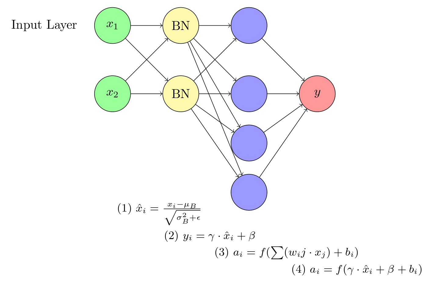
A visual representation of a neural network incorporating Batch Normalization (BN). The network consists of an input layer, a hidden layer, and an output layer. The BN layer is positioned between the input and hidden layers, normalizing the input data and improving the overall training efficiency.
How does Batch Normalization work?
Batch normalization is a widely used technique in the field of machine learning that improves the speed of neural network training while providing regularization to avoid overfitting. In simple terms, it standardize the inputs to layers in a neural network. The technique was introduced to address the problem of internal covariate shift, which arises due to updating multiple-layer inputs simultaneously in deep neural networks.
During training, batch normalization replaces the i-th hidden layer of a vanilla network with a batch normalization layer. This layer applies a linear transformation to the input values, followed by rescaling and offsetting. The rescaling and offsetting parameters are learned during training, and they help to smooth the loss function, speed up the training process, and handle internal covariate shifts.
Internal Covariate Shifts
Covariate shift is a common issue in machine learning, where the training and test sets have different distributions, making it difficult for the model to generalize well. While standardization and whitening techniques can help, they can be computationally intensive and not ideal for real-time applications.
Internal covariate shift occurs when network activations change between layers during training. Ideally, we want each layer’s distribution to be consistent while maintaining functional relationships. To avoid complex calculations, the input features are normalized within each layer and mini-batch, ensuring a mean of zero and a standard deviation of one. This makes it more efficient and practical for real-world applications.
Normalization of the Input
The normalization step calculates the mean and standard deviation of the previous layers’ outputs and normalizes them, making them easier to train. The rescaling and offsetting steps add non-linearity to the network and prevent saturation of the sigmoid functions in the network.
Batch normalization can be implemented in various deep learning frameworks like Keras, PyTorch, and TensorFlow. It has numerous applications in deep learning, including image recognition, natural language processing, and speech recognition.
The first step in batch normalization is to normalize the input to each layer. Let’s consider a mini-batch of size m, which is fed into a layer of a neural network. The input to the layer can be represented as x = [x1, x2, …, xm], where xi is the input to the i-th instance in the mini-batch. The mean and variance of the input can be computed as follows:
μ = (1/m) * Σxi
Latex: \mu_B = \frac{1}{m} \sum_{i=1}^{m} x_i (1)

σ^2 = (1/m) * Σ(xi-μ)^2
Latex: \sigma_B^2 = \frac{1}{m} \sum_{i=1}^{m} (x_i - \mu_B)^2 (2)
Here, μ is the mean of the input, σ^2 is the variance of the input, and Σ is the summation of all the inputs in the mini-batch.
The normalized input can be represented as follows:
x̂ = (x - μ) / √(σ^2 + ε)

Latex: \hat{x}_i = \frac{x_i - \mu_B}{\sqrt{\sigma_B^2 + \epsilon}} (3)
Here, ε is a small constant (e.g., 10^-5) added to the variance for numerical stability.
Rescaling of Offsetting
The normalized input x̂ is rescaled and offset using two learnable parameters, γ and β, respectively. These parameters are learned during training and used to transform the normalized input x̂ into the output y as follows:
y = γ * x̂ + β
Latex: y_i = \gamma \hat{x}_i + \beta (4)
Equation (4) scales and shifts the normalized input x̂i using learnable parameters γ and β, which are updated during the training process. The result is the output yi of the Batch Normalization layer.
Incorporating Batch Normalization into Neural Network Node Equations
We will now explore how the equations for batch normalization are incorporated into neural network node equations and how it influences the training process.
Neural networks consist of interconnected nodes or neurons, where each node computes a weighted sum of its inputs, adds a bias term, and then applies an activation function. The equation for a typical node i in a neural network without batch normalization is:
a_i = f(Σ(w_ij * x_j) + b_i) (5)
Here, a_i is the activation of the i-th node, f is the activation function, w_ij is the weight connecting node j to node i, x_j is the input from node j, and b_i is the bias term for the i-th node.
To incorporate batch normalization, we first normalize the weighted sum (Σ(w_ij * x_j)) before applying the activation function. We replace the weighted sum in Equation (5) with the output y from Equation (4). The modified node equation with batch normalization becomes:
a_i = f(γ * x̂_i + β + b_i) (6)
In this modified node equation, the input x̂_i is normalized using Equations (1), (2), and (3), and then rescaled and offset using Equation (4). The learnable parameters γ and β help preserve the non-linearity of the network and counteract any potential saturation in the activation functions.
Also Read: Introduction to Radial Bias Function Networks
Advantages of Batch Normalization
Faster Training Speed: Batch normalization helps to speed up the training process by normalizing the hidden layer activations and smoothing the loss function. This ensures that the model converges quickly and efficiently. It also allows for higher learning rates, which helps to speed up the training process. This is because gradient descent usually requires small learning rates for the network to converge, but batch normalization allows us to use much higher learning rates.

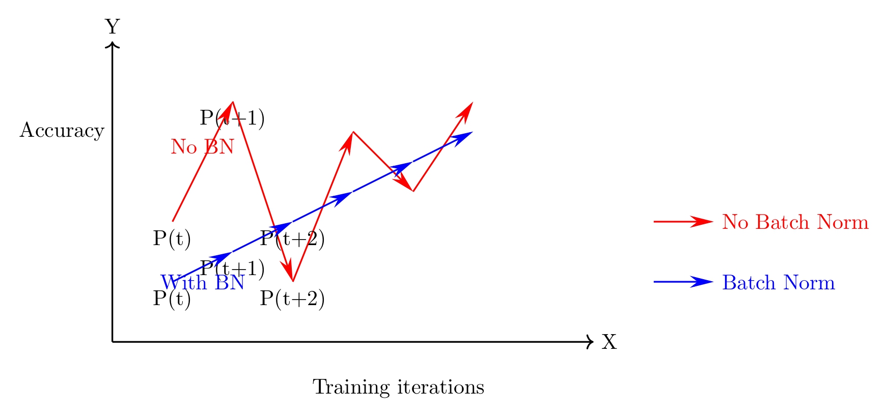
Comparison of training trajectories with and without Batch Normalization: The plot illustrates how the application of Batch Normalization (blue) leads to smoother and more consistent improvements in accuracy across training iterations compared to training without Batch Normalization (red).
Handles Internal Covariate Shift
In the original paper by Sergey and Christian, it is claimed that Batch Normalization reduces the internal covariate shift of the network. This refers to the phenomenon where the distribution of activations in a layer changes during training, which can slow down the learning process. Batch Normalization addresses this issue by normalizing the activations using the mean and variance of the current mini-batch, which helps to stabilize the distribution of activations and speeds up training. This eliminates the need for the model to constantly update its parameters based on changes in the distribution of input data.
Easier Weight Initialization
Batch normalization makes weight initialization easier by allowing us to be less careful when choosing our initial starting weights especially when creating deeper networks. The initial values of weights play a significant role in the performance of batch normalization. With the right method of batch normalization, improvements in the learning algorithm can be achieved, leading to the success of the technique.
Provides Regularization
Batch normalization adds a little noise to the network, which can act as a form of regularization. In some cases, it has been shown to work as well as dropout, which is a common regularization technique. However, it’s important to note that relying solely on batch normalization for regularization can lead to issues with module orthogonality, where one module should ideally address one specific issue. It’s recommended to use other regularization techniques in addition to batch normalization to ensure the best possible performance and avoid unnecessary development complexities.
Batch Normalization Python Implementation
The performance of a neural network hinges on factors such as gradient magnitude and the implementation of various gradient descent techniques, including full-batch, mini-batch, and regular gradient descent. Optimizing these aspects contributes to more efficient training and improved model performance, especially when combined with advanced techniques such as batch normalization.
The leading deep learning frameworks, including PyTorch, TensorFlow, and Keras, all provide implementations of batch normalization layers. These implementations simplify the integration of batch normalization into your models, allowing you to configure settings independently.
The PyTorch framework offers torch.nn.BatchNorm1d, torch.nn.BatchNorm2d, and torch.nn.BatchNorm3dfor implementing batch normalization in 1D, 2D, and 3D networks, respectively.
In the TensorFlow/Keras framework, you can utilize tf.nn.batch_normalization or tf.keras.layers.BatchNormalization for implementing batch normalization.
When implementing batch normalization, it is vital to set the input vector size according to the number of neurons or filters in the current hidden layer. For multi-layer perceptrons (MLP), this size depends on the number of neurons, while for convolutional networks, it is determined by the number of filters. Proper configuration of the input vector size is essential for achieving optimal performance in deep learning models incorporating batch normalization.
Batch Normalization using Pytorch
The BatchNorm2d class in PyTorch applies Batch Normalization on 4D inputs (mini-batches of 2D inputs with an additional channel dimension) as proposed in the paper “Batch Normalization: Accelerating Deep Network Training by Reducing Internal Covariate Shift.”
torch.nn.BatchNorm2d(num_features, eps=1e-05, momentum=0.1,
affine=True, track_running_stats=True, device=None, dtype=None)
This class calculates the mean and standard deviation per dimension over mini-batches, with learnable parameter vectors γ and β (default: γ elements are set to 1, β elements set to 0). The layer maintains running estimates of mean and variance during training (default momentum: 0.1), which are used for normalization during evaluation. This process is commonly called Spatial Batch Normalization.
Parameters like num_features, eps, momentum, affine, and track_running_stats can be adjusted to modify the behavior of the BatchNorm2d class. The input and output shapes are the same, and the class can be easily integrated into a deep learning model to accelerate training and improve performance.
Batch Normalization using Tensorflow & Keras
Below is BatchNormalization class, found within Keras, a TensorFlow submodule It keeps the mean output near zero and the standard deviation close to one. Interestingly, it behaves differently during the training and inference phases. While training, the layer uses the mean and standard deviation of the current batch. During inference, however, it relies on a moving average from batches encountered during training.
The class offers various adjustable parameters, such as axis, momentum, epsilon, center, and scale, among others. Including this layer in deep learning, models can enhance training speed and the model’s overall performance.
tf.keras.layers.BatchNormalization( axis=-1, momentum=0.99, epsilon=0.001, center=True,
scale=True, beta_initializer="zeros", gamma_initializer="ones", moving_mean_initializer="zeros", moving_variance_initializer="ones",
beta_regularizer=None,
gamma_regularizer=None,
beta_constraint=None,
gamma_constraint=None,
synchronized=False,
**kwargs
)
In this code snippet below, we have demonstrated the effectiveness of using Batch Normalization (BN) in a neural network. The code is divided into several parts:
1) Defining a function create_model(use_bn=False) to create a neural network with or without Batch Normalization. The model consists of a Flatten layer, ReLU activation, a Dense layer with 128 neurons, an optional BN layer, and an output Dense layer with 10 neurons. The model is compiled using the Adam optimizer and sparse categorical cross-entropy loss.
import tensorflow as tf
import matplotlib.pyplot as plt

# Create the neural network model with and without BN
def create_model(use_bn=False):
model = tf.keras.Sequential()
model.add(tf.keras.layers.Flatten(input_shape=(28, 28)))
model.add(tf.keras.layers.Dense(128, activation='relu'))
if use_bn:
model.add(tf.keras.layers.BatchNormalization())
model.add(tf.keras.layers.Dense(10, activation='softmax'))
model.compile(optimizer='adam', loss='sparse_categorical_crossentropy', metrics=['accuracy'])
return model
2) Loading and preprocessing the MNIST dataset, which contains grayscale images of handwritten digits. And finally training two models: one without Batch Normalization and the other with Batch Normalization. Both models are trained for 10 epochs, with a 20% validation split.
# Load and preprocess the dataset
(x_train, y_train), (x_test, y_test) = tf.keras.datasets.mnist.load_data()
x_train, x_test = x_train / 255.0, x_test / 255.0

# Train the models
model_no_bn = create_model(use_bn=False)
history_no_bn = model_no_bn.fit(x_train, y_train, epochs=10, validation_split=0.2, verbose=0)

model_bn = create_model(use_bn=True)
history_bn = model_bn.fit(x_train, y_train, epochs=10, validation_split=0.2, verbose=0)
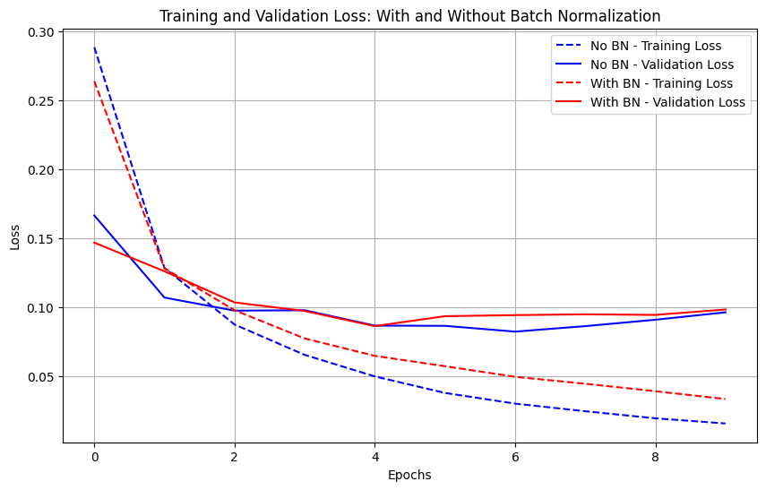
3) Plotting the training and validation losses for both models, comparing the performance of the models with and without Batch Normalization. We can observe Batch normalization leads to faster convergence and lower validation loss, showcasing the effectiveness in improving the model’s performance and generalization capabilities.
# Plot the comparison
plt.figure(figsize=(10, 6))
plt.plot(history_no_bn.history['loss'], label='No BN - Training Loss', linestyle='--', color='blue')
plt.plot(history_no_bn.history['val_loss'], label='No BN - Validation Loss', linestyle='-', color='blue')
plt.plot(history_bn.history['loss'], label='With BN - Training Loss', linestyle='--', color='red')
plt.plot(history_bn.history['val_loss'], label='With BN - Validation Loss', linestyle='-', color='red')

plt.xlabel('Epochs')
plt.ylabel('Loss')
plt.title('Training and Validation Loss: With and Without Batch Normalization')
plt.legend()
plt.grid()
plt.show()
Effect of Batch Normalization on Neural Network Performance: A Comparative Analysis of Training and Validation Loss
Challenges of Batch Normalization
Batch normalization is a powerful tool in deep learning, but it also has its limitations and challenges that must be addressed. Here are some of the main challenges associated with batch normalization:
Small Batch Sizes
Batch normalization relies on sample statistics like mean and standard deviation to normalize the data. However, when the Mini – Batch size is small, these statistics may not be representative of the entire dataset, leading to poor performance. For instance, when the mini- batch size is too small, usually 1, it can lead to unsatisfactory results. Moreover, Batch normalization is highly dependent on the mini-batch size and can converge to different solutions, which can impact the overall performance of the model. To address this issue, using larger batch sizes or alternative normalization methods like layer normalization or instance normalization can be useful.
Sequence Models
In sequence models like RNNs, the input varies in length, making it difficult to apply batch normalization. This is because the statistics of each sequence may be different, and therefore the normalization parameters cannot be easily shared across all sequences. To overcome this challenge, several normalization techniques have been proposed, including batch renormalization, weight normalization, and layer normalization.
Impact on Model Interpretability
Batch normalization can make it harder to interpret the model as it adds an extra layer of complexity. The normalized values can also make it difficult to understand the true impact of each feature on the final output. To address this, alternative normalization techniques that preserve interpretability like feature-wise normalization can be used.
Computation Overhead
Batch normalization requires additional computations during both the forward and backward passes, resulting in slower training and longer inference times, especially on low-power devices like mobile phones. To address this, optimization techniques like fused batch normalization that combine batch normalization with other layers to reduce computation overhead can be used.
Recent Advances in Batch Normalization
Recent advances in normalization methods have focused on improving the performance and stability of deep neural network (DNN) optimization. One study introduced a new normalization layer called Batch Layer Normalization (BLN), which combines batch and layer normalization to adaptively weight mini-batch and feature normalization based on the inverse size of mini-batches during the learning process. BLN was found to have faster convergence than traditional batch and layer normalization methods in both Convolutional and Recurrent Neural Networks.
Another recent paper proposed a refinement of Batch Normalization called Full Normalization (FN), which addresses issues with Batch Normalization when batches are not constructed ideally. FN uses a compositional optimization technique to create a new objective function that improves the performance of BN.
Finally, researchers have also highlighted the importance of understanding the limitations of Batch Normalization, such as poor performance when batch size is small and dependence on ideal batch statistics. Corrected formulations of Batch Normalization have been proposed to address these issues and improve inference performance. These recent advances offer promising new directions for improving normalization methods in DNNs.
Conclusion
In wrapping up, batch normalization has emerged as a game-changing technique in the realm of deep neural networks, effectively tackling obstacles like internal covariate shifts, sluggish convergence, and overfitting. This approach standardizes inputs to network layers, enabling faster training, better model performance, and providing inherent regularization.
However, it is essential to be aware of its challenges, such as small batch sizes, sequence models, model interpretability, and computational overhead. Researchers continue to explore advances in normalization techniques to overcome these challenges and further enhance performance.
References
BatchNorm2d — PyTorch 2.0 Documentation. https://pytorch.org/docs/stable/generated/torch.nn.BatchNorm2d.html. Accessed 21 Apr. 2023.
Ioffe, Sergey, and Christian Szegedy. “Batch Normalization: Accelerating Deep Network Training by Reducing Internal Covariate Shift.” arXiv.Org, 11 Feb. 2015, https://arxiv.org/abs/1502.03167. Accessed 21 Apr. 2023.
Team, Keras. Keras Documentation: BatchNormalization Layer. https://keras.io/api/layers/normalization_layers/batch_normalization/. Accessed 21 Apr. 2023.
“Two Recent Advances on Normalization Methods for Deep Neural Network Optimization.” IEEE Xplore, https://ieeexplore.ieee.org/document/9301751. Accessed 21 Apr. 2023.
Ziaee, Amir, and Erion Çano. “Batch Layer Normalization, A New Normalization Layer for CNNs and RNN.” arXiv.Org, 19 Sept. 2022, https://arxiv.org/abs/2209.08898. Accessed 21 Apr. 2023.


