Introduction
Orthonormal vectors are a set of vectors that are both orthogonal (perpendicular) to each other and have a unit length (norm) of 1. In other words, the dot product of any two distinct vectors in the set is zero, and the dot product of a vector with itself is 1. Orthonormal vectors play a crucial role in machine learning, particularly in the context of dimensionality reduction and feature extraction. Techniques such as Principal Component Analysis (PCA) rely on finding orthonormal bases that can optimally represent the variance in the data, enabling efficient compression and noise reduction.
Additionally, orthonormal vectors are used in various machine learning algorithms to simplify computations, improve numerical stability, and facilitate the interpretation of results. Their orthogonal nature ensures that the dimensions in the transformed space are independent and uncorrelated, which is often a desirable property in machine learning models.
Linear algebra, which deals with vectors and matrices, is one of the fundamental branches of mathematics for machine learning. Vectors are often used to represent data points or features, while matrices are used to represent collections of data points or sets of features. In image recognition tasks, an image can be represented as a vector of pixel values, and a set of images can be represented as a matrix where each row corresponds to an image vector.
By using vectors to represent data, machine learning or deep learning algorithms can apply mathematical operations such as matrix multiplication and dot products to manipulate and analyze the data. For example, vector operations such as cosine similarity can be used to measure the similarity between two data points or to project high-dimensional data onto a lower-dimensional space for visualization or analysis. By grouping similar vectors together or predicting the value of a target variable based on the values of other variables, these algorithms can make predictions or identify patterns in the data.
There are different types of vectors such as orthogonal vector, orthonormal vector, column vector, row vector, dimensional feature vector, independent vector, resultant feature vector, etc.
The difference between a column vector and a row vector is primarily a matter of convention and notation. In most cases, the choice of whether to use a column vector or a row vector depends on the context and the specific application.
Dimensional feature vector is a representation of an object or entity that captures relevant information about its properties and characteristics in a multidimensional space. In other words, it is a set of features or attributes that describe an object, and each feature is assigned a value in a numerical vector.
A vector is considered an independent vector if no vector can be expressed as a linear combination of those listed before it in the set. independent vector independent vector.
Resultant feature vector is a vector that summarizes or combines multiple feature vectors into a single vector that captures the most important information from the original vectors. The process of combining feature vectors is called feature aggregation, and it is often used in machine learning and data analysis applications where multiple sources of information need to be combined to make a decision or prediction. Resultant feature vectors can be useful in reducing the dimensionality of data and in summarizing complex information into a more manageable form. They are widely used in applications such as image and speech recognition, natural language processing, and recommendation systems.
Table of contents
Also Read: What is a Sparse Matrix? How is it Used in Machine Learning?
Orthogonal and Orthonormal Vectors
In the context of data analysis and modeling, it can be useful to transform the original variables or input variables into a new set of variables that are orthogonal or orthonormal. Explanatory variables can be thought of as the components of the vector that are used to explain or predict a response variable and its components can be thought of as quantitative variables.
Orthogonal and orthonormal vector algorithms play an important in machine learning because they enable efficient computations, simplify many mathematical operations, and can improve the performance of many machine learning algorithms.
What are orthogonal vectors?
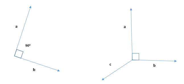
The word orthogonal comes from the Greek meaning “right-angled”. An orthogonal vector is a vector that is perpendicular to another vector or set of vectors. In other words, the dot product of two orthogonal vectors is zero, which means that they have no component in the same direction.
For example, in two-dimensional space, the vector (1, 0) is orthogonal to the vector (0, 1), since their dot product is 10 + 01 = 0. Similarly, in three-dimensional space, the vector (1, 0, 0) is orthogonal to both (0, 1, 0) and (0, 0, 1).

2D and 3D Orthogonal Vector
Orthogonal vectors are often used in linear algebra, where they are used to construct orthogonal bases for vector spaces, which can simplify calculations and make them more efficient. Linear combinations of vectors are also used frequently in linear algebra, where they can be used to represent any vector in a given space as a linear combination of a set of basis vectors.
It’s important to note that normal vector and orthogonal vector is often used interchangeably to refer to a vector that is perpendicular to another vector or surface, however there is a subtle difference between the two concepts. Normal vector is typically used to describe a vector that is perpendicular to a surface while orthogonal vector is more general and can refer to any two vectors that are perpendicular to each other.
In machine learning, linear combinations of orthogonal vectors are used in various ways, such as in dimensionality reduction techniques like Principal Component Analysis (PCA). By using linear combinations of orthogonal vectors to represent the data, we can achieve a more efficient and effective representation that captures the most important aspects of the data, while reducing noise and redundancy. This can improve the performance of machine learning algorithms by reducing overfitting, improving generalization, and reducing computational complexity. In pattern recognition, orthogonal vectors are used in various ways, such as in feature extraction and classification algorithms.
Also Read: Introduction to Vector Norms: L0, L1, L2, L-Infinity
Orthogonal matrices
An orthogonal matrix is a square matrix whose columns and rows are orthogonal to each other. Square matrix means the number of rows and columns is the same. It is a special type of matrix that makes use of transposes and inverses. A reflection matrix is a particular type of orthogonal matrix that describes a reflection of a vector or a point across a given line or plane. A reflection matrix is symmetric, meaning that it is equal to its transpose.
Geometrically, an orthogonal matrix preserves the length and angle between vectors. This means that when an orthogonal matrix is applied to a vector, the resulting vector is rotated and/or reflected in a way that preserves its length and angle with respect to other vectors.
There are several interesting properties of orthogonal matrices
- Its transpose is equal to its inverse of matrix. The inverse of matrix is a matrix that, when multiplied by the original matrix, gives the identity matrix as the result.
- Product of an orthogonal matrix with its transpose gives an identity matrix. In other words, if A is an orthogonal matrix, then A^T * A = A * A^T = I, where I is the identity matrix.
- The transpose of an orthogonal matrix is also always orthogonal
- The largest eigenvalue of an orthogonal matrix is always 1 or -1, because the product of the eigenvalues of an orthogonal matrix is equal to the determinant, which for an orthogonal matrix is either 1 or -1.
Orthogonal matrices and matrix norms are an important concept in linear algebra and matrix factorization. Matrix norm are used to measure the size of a matrix or a vector, which can be helpful in regularization and avoiding overfitting. Matrix factorization is a technique in linear algebra that involves decomposing a matrix into a product of simpler matrices. The goal of matrix factorization is often to represent the original matrix in a more compact form that is easier to analyze or manipulate. Other matrix factorization techniques, such as QR factorization and Cholesky decomposition, also involve finding sets of orthogonal vectors that can be used to simplify the matrix representation. They are used in a variety of applications, including computer graphics, physics, engineering, and cryptography.
It is also interesting to explore the relation between orthogonal matrix and other types of matrices relevant to machine learning such as unitary matrix, diagonal matrix, triangular matrix, symmetric matrix and score matrix.
Unitary matrix
A unitary matrix, is a complex square matrix where the columns are all unitary vectors, meaning that they are orthogonal to each other and have a length of one in the complex sense. In other words, if U is a unitary matrix, then U^H * U = U * U^H = I, where U^H is the Hermitian transpose of U. The relationship between orthogonal matrices and unitary matrices is that every orthogonal matrix is a real-valued unitary matrix. This means that if A is an orthogonal matrix, then it is also a unitary matrix when viewed as a complex matrix with zeros in the imaginary part. Conversely, every unitary matrix with real entries is an orthogonal matrix.In deep learning, unitary matrices are used in various contexts, such as in the design of neural networks and in the computation of quantum-inspired algorithms.
Unitary matrices are important in many areas of machine learning, such as:
- Singular Value Decomposition (SVD): In Singular Value Decomposition, a matrix is factorized into three matrices, one of which is a unitary matrix. This unitary matrix represents the rotation or transformation of the original data.
- Signal processing: Unitary matrices can be used for Fourier analysis, which is a technique used in signal processing to decompose a signal into its frequency components.
Diagonal matrix
A diagonal matrix is a square matrix where all the off-diagonal elements are zero, and the diagonal elements can be any value. An example of a diagonal matrix is the matrix of eigenvalues in eigendecomposition. The relationship between orthogonal matrix and diagonal matrix is that every orthogonal matrix can be decomposed into a product of a diagonal matrix and an orthogonal matrix that is its transpose. This decomposition is known as the singular value decomposition (SVD), and it can be written as follows:
A = U * D * V^T
Where A is the orthogonal matrix, U and V are orthogonal matrices, and D is a diagonal matrix. The columns of U and V are the left and right singular vectors of A, respectively, and the diagonal elements of D are the singular values of A. The Singular Value Decomposition is a powerful tool in linear algebra and machine learning, as it can be used for various tasks such as dimensionality reduction, matrix compression, and matrix inversion.
Diagonal matrices are used in various areas of machine learning, such as:
- Principal Component Analysis (PCA): Linear combinations of orthogonal vectors are often used as a way of representing data in a lower-dimensional space, a technique known as principal component analysis (PCA). The key concepts in PCA include orthogonal vectors, standard deviation, squared error, correlation matrix, eigenvalues and eigenvectors. The original variables are transformed into a set of orthonormal variables and the covariance matrix is diagonalized to find the principal components. This diagonalization is done by finding the eigenvectors and eigenvalues of the covariance matrix, which is often a symmetric positive-definite matrix.
- Regularization: In regularization, diagonal matrices are added to the original matrix to prevent overfitting. These diagonal matrices are often referred to as “penalty” or “shrinkage” terms.
- Transformation: Diagonal matrices can be used to transform a dataset. For example, in signal processing, diagonal matrices can be used to represent filters.
Triangular matrix
A triangular matrix is a square matrix where all the elements above or below the main diagonal are zero. The main diagonal is the line that runs from the top-left corner of the matrix to the bottom-right corner. Every orthogonal matrix can be decomposed into a product of a triangular matrix and an orthogonal matrix: Any square matrix can be decomposed into a product of a lower triangular matrix and an upper triangular matrix. In the case of an orthogonal matrix, we can decompose it into a product of a lower triangular matrix and an orthogonal matrix by using the Gram-Schmidt process. This decomposition is called QR factorization, where Q is an orthogonal matrix and R is an upper triangular matrix.
These relationships between orthogonal matrices and triangular matrices are important in many areas of mathematics and engineering, including linear regression, signal processing, and numerical linear algebra.
Symmetric matrix
A symmetric matrix is a square matrix where the elements above and below the diagonal are mirror images of each other. In other words, A[i,j] = A[j,i] for all i and j. A symmetric matrix is always diagonalizable, which means that it can be decomposed into a product of its eigenvectors and eigenvalues. The connection between orthogonal and symmetric matrices is that if A is a symmetric matrix, then its eigenvectors are orthogonal to each other. Furthermore, the eigenvectors of a symmetric matrix can be chosen to be orthonormal, which means that they are orthogonal to each other and have a length of one. In other words, the eigenvectors of a symmetric matrix form an orthonormal basis. This connection between orthogonal and symmetric matrices is useful in many areas of deep learning where symmetric matrices arise frequently.
This makes them particularly useful in many applications, such as principal component analysis and spectral clustering.
Score matrix
A score matrix is a matrix that is used to assign scores or penalties to pairs of sequences in a sequence alignment. Score matrices are used in bioinformatics and computational biology to score sequence alignments based on their similarity. Orthogonal matrices can be used in certain applications related to sequence alignment and score matrices. For example, in some methods for calculating the optimal sequence alignment score using dynamic programming, the algorithm involves calculating the score matrix recursively. The matrix multiplication step involved in this algorithm can be seen as equivalent to transforming one score matrix into another using an orthogonal matrix.
Also Read: PCA-Whitening vs ZCA Whitening: What is the Difference?
What are orthonormal vectors?
An orthonormal vector is a vector that has a magnitude (length) of 1 and is perpendicular (orthogonal) to all other vectors in a given set of vectors. In other words, a set of orthonormal vectors forms an orthogonal basis for the vector space in which they reside. The term “ortho” comes from the Greek word for “perpendicular,” while “normal” is used to indicate that the vectors have a length of 1, which is also referred to as being normalized. It is also known as an orthogonal unit vector.
A set of vectors {v1, v2, …, vn} is orthonormal if:
- Each vector vi is a unit vector, meaning that ||vi|| = 1.
- Each vector vi is orthogonal to every other vector vj, where i and j are distinct indices.
In linear algebra, orthonormal vectors are often used to simplify calculations and represent geometric concepts. They are commonly used in applications such as computer graphics, signal processing, and quantum mechanics, among others. In pattern recognition, orthonormal vectors are used in various ways, such as in dimensionality reduction, feature extraction, and classification algorithms. Some algorithms that employ orthogonal vectors include Singular Value Decomposition (SVD). SVD is a popular method used for dimensionality reduction and Haar Transform, a method used for compressing digital images.
Visualization of Orthogonal Vectors
To visualize orthogonal vectors, we can use a 2D or 3D coordinate system.
In 2D, we can imagine two vectors that are perpendicular to each other, with one vector pointing horizontally (along the x-axis) and the other pointing vertically (along the y-axis). The two vectors form a right angle at the origin of the coordinate system.
Python code
#matplotib and numpy import
import matplotlib.pyplot as plt
import numpy as np

fig = plt.figure(figsize=(4, 4))
ax = fig.add_subplot(111)

ax.grid(alpha=0.4)
ax.set(xlim=(-3, 3), ylim=(-3, 3))

#numpy import array
v1 = np.array([1, 2])
v2 = np.array([2, -1])

# Plot the orthogonal vectors
ax.annotate('', xy=v1, xytext=(0, 0), arrowprops=dict(facecolor='b'))
ax.annotate('', xy=v2, xytext=(0, 0), arrowprops=dict(facecolor='g'))

plt.show()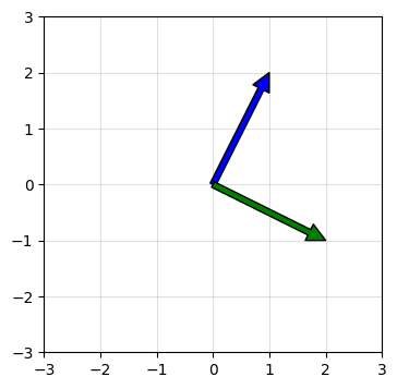
In 3D, we can imagine three vectors that are mutually orthogonal to each other. We can visualize this by drawing three axes: the x-axis, y-axis, and z-axis. The three axes form a right-handed coordinate system. The vector along the x-axis is orthogonal to both the y-axis and the z-axis, the vector along the y-axis is orthogonal to both the x-axis and the z-axis, and the vector along the z-axis is orthogonal to both the x-axis and the y-axis.
Python code
#matplotib and numpy import
import matplotlib.pyplot as plt
import numpy as np

fig = plt.figure(figsize=(7,7))
ax = fig.add_subplot(111, projection="3d")

#Define the orthogonal vectors
#numpy import array
v1 = np.array([0, 0, -1])
v2 = np.array([1, 1, 0])
v3 = np.array([-1, 1, 0])

# Plot the orthogonal vectors
ax.quiver(0,0,0, v1[0], v1[1], v1[2], color='r', lw=3, arrow_length_ratio=0.2)
ax.quiver(0,0,0, v2[0], v2[1], v2[2], color='g', lw=3, arrow_length_ratio=0.2)
ax.quiver(0,0,0, v3[0], v3[1], v3[2], color='b', lw=3, arrow_length_ratio=0.2)

ax.set_xlim([-1, 1]), ax.set_ylim([-1, 1]), ax.set_zlim([-1, 1])
ax.set_xlabel('X axis'), ax.set_ylabel('Y axis'), ax.set_zlabel('Z axis')
plt.show()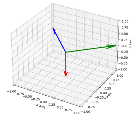
We can also use geometric shapes to visualize orthogonal vectors. For example, in 2D, we can draw a rectangle with sides parallel to the x-axis and y-axis. The sides of the rectangle represent the orthogonal vectors. Similarly, in 3D, we can draw a rectangular prism with sides parallel to the x-axis, y-axis, and z-axis. The edges of the rectangular prism represent the orthogonal vectors.
Also Read: How to Use Linear Regression in Machine Learning.
Orthogonal Vectors Histogram (OVH)
An orthogonal vector histogram is a way to represent a set of vectors in a high-dimensional space. The basic idea behind an orthogonal vector histogram is to partition the space into a set of orthogonal subspaces and then count the number of vectors that lie within each subspace.
To create an orthogonal vector histogram, we first choose a set of orthogonal basis vectors that span the space. For example, in 3D space, we might choose the three unit vectors along the x, y, and z axes. Next, we divide each axis into a set of bins or intervals, and we count the number of unit vectors that fall into each bin. For example, if we divide each axis into 10 bins, we would count the number of vectors that fall into each of the 10 x-bins, each of the 10 y-bins, and each of the 10 z-bins.Finally, we represent the counts in a histogram or bar chart, with each bin or interval along each axis corresponding to a bar in the chart.The resulting histogram provides a visualization of the distribution of vectors in the high-dimensional space, with each bar representing the number of vectors that fall into a particular region of the space. The use of orthogonal subspaces and bins allows us to represent complex distributions in a simple and intuitive way.
Orthogonal vector histograms are a powerful technique for pattern recognition and classification. In pattern recognition, the goal is to identify and categorize objects based on their underlying features, such as shape, color, texture, or orientation. Orthogonal vector histograms can be used to extract and represent these features in a high-dimensional space, allowing us to compare and classify objects based on their similarity in this space. OVH can be used in image classification tasks as a way to represent image features in a high-dimensional space. In this context, each image can be represented as a set of vectors, where each vector corresponds to a particular feature of the image. To create an orthogonal vector histogram for an image, we first extract a set of features from the image using techniques such as edge detection, texture analysis, or color histogramming. Each feature is then represented as a vector in a high-dimensional space, with each dimension corresponding to a particular aspect of the feature (e.g., orientation, texture, color). We can then create an orthogonal vector histogram by dividing the high-dimensional space into a set of orthogonal subspaces and counting the number of feature vectors that fall into each subspace. The resulting histogram provides a compact representation of the image features, capturing the essential information needed for image classification.
Implementation details
In computer vision, labeling images into semantic categories is a challenging problem to solve. Image classification is a challenging task because of several characteristics associated with the image such as illumination, clutter, partial occlusion and others. Bag of visual words (BOVW) is a widely used machine learning model in image classification. Its concept is adapted from NLP’s bag of words (BOW) where we count the number of times each word appears in a document, use the frequency of the words to determine the keywords and make a frequency histogram. It does not retain the order of the words. In BoVW model, the local features are quantized and 2-D image space is represented in the form of order-less histogram of visual words but the image classification performance suffers due to the order-less representation of image.
A research published in the doi journal presented a novel way to model global relative spatial orientation of visual words in a rotation invariant manner which demonstrated remarkable gain in the classification accuracy over the state-of-the-art methods. Four image benchmarks were used to validate the approach.
The figure and the details that follow describes the approach:
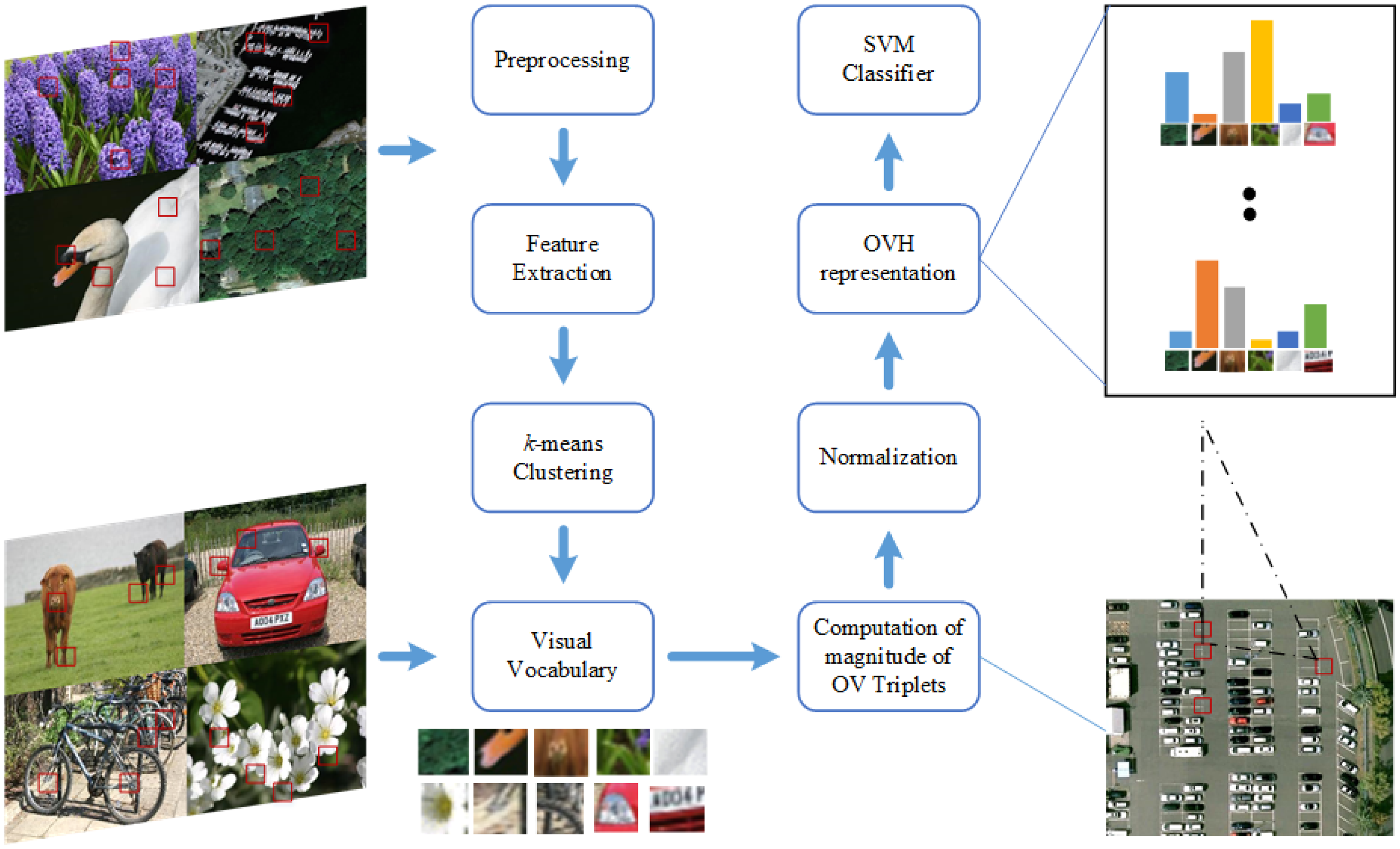
Block diagram of proposed research based on OVH
Source: doi
- Pre-processing step – large images are resized to a standard size of 480 × 480 pixels.
- Feature extraction – all images are converted to gray scale.
- K-means clustering – is used to generate the visual vocabulary. Since K-means is unsupervised, the experiment is repeated multiple times with random selection of training and test images.
- OV triplets – A threshold and a random selection is used to limit the number of words of the same type used for the creating triplet combinations.
- OVH representation – A 5-bin OVH representation for the results is presented.
- Classification – Support Vector Machines (SVM) is used for classification. Kernel method is used to generate non-linear decision boundaries. The resulting histogram is normalized and SVM Hellinger Kernel is applied because of its low compute cost. SVM Hellinger kernel can explicitly compute the features map instead of computing the kernel values and the classifier remains linear. A 10-fold cross validation is applied on the training dataset to determine the optimal value. The one-against-one approach is applied. In this approach, a binary classifier is trained for each possible pair of classes in the dataset. One advantage of the one-against-one approach is that it can be more computationally efficient than other approaches, especially when there are many classes.
The four standard image benchmarks included the following datasets:
- 15-scene image dataset – comprised a wide range of indoor and outdoor category images including personal photographs, the Internet and COREL collections. The dataset included 4485 images with an average image size 300 × 250 pixels.
- MSRC-v2 image dataset – consisted of 591 images classified into 23 categories. The objects exhibited intra-class variation in shape and size, in addition to partial occlusion.
- UC Merced land-use (UCM) image dataset – comprised 21 land-use classes from the United States Geological Survey (USGS) National map. Each class contained 100 images of size 256 × 256 pixels providing large geographical scale.
- 19-class satellite scene image dataset – comprised 19 high-resolution satellite scene categories with a focus on This dataset focused on images with a large geographical scale and contained at least 50 images/class, size 600 × 600 pixels.
The results successfully incorporated relative global spatial information into the BoVW model. The proposed approach outperformed other concurrent local and global histogram based methods and provided a competitive performance.
Also Read: What Are Support Vector Machines (SVM) In Machine Learning
Conclusion and future directions
Orthogonal vectors and histograms are a powerful tool in pattern recognition, as they enable us to identify the most informative features, separate the different classes, and cluster the data in an efficient and effective way. Overall, orthogonal vector histograms provide a powerful and flexible way to represent image features, and can be used in a wide range of image classification tasks, including object recognition, scene classification, and face recognition.

References
Image classification by addition of spatial information based on histograms of orthogonal vectors https://doi.org/10.1371/journal.pone.0198175. Accessed 30 Mar. 2023
Vedaldi A, Zisserman A. Sparse kernel approximations for efficient classification and detection. In: Computer Vision and Pattern Recognition (CVPR), 2012 IEEE Conference on. IEEE; 2012. p. 2320–2327. Accessed 30 Mar. 2023
Fatih Karabiber, “Orthogonal and Orthonormal Vectors”, https://www.learndatasci.com/glossary/orthogonal-and-orthonormal-vectors. Accessed 1 Apr. 2023
Ali N, Bajwa KB, Sablatnig R, Chatzichristofis SA, Iqbal Z, Rashid M, et al. “A Novel Image Retrieval Based on Visual Words Integration of SIFT and SURF”, https://journals.plos.org/plosone/article?id=10.1371/journal.pone.0157428. Accessed 30 Mar. 2023
Bethea Davida, “Bag of Visual Words in a Nutshell”, https://towardsdatascience.com/bag-of-visual-words-in-a-nutshell-9ceea97ce0fb. Accessed 1 Apr. 2023
Chatzichristofis SA, Iakovidou C, Boutalis Y, Marques O. Co. vi. wo.: color visual words based on non-predefined size codebooks. IEEE transactions on cybernetics. 2013;43(1):192–205. pmid:22773049. Accessed 2 Apr. 2023