Vector Norms Explained: L0, L1, L2, and L-Infinity (With Formulas and Examples)

Introduction

Almost every model you touch leans on vector norms without ever announcing it. A norm is the rule that collapses a whole list of numbers into one honest measure of size. That single number then steers optimization, regularization, similarity, and distance across machine learning. The classic deep learning text by Goodfellow and colleagues introduces them within its opening chapters. The L1, L2, and L-infinity norms each judge magnitude by a different rule, and that rule quietly shapes results. Choose poorly and you can waste compute, smear useful signal, or send a training run off a cliff. This guide walks through the four most common vector norms with plain definitions, formulas, and worked numbers. By the final section you will know which measure fits which job and why.

Quick Answers on Vector Norms

What are vector norms, briefly?

Vector norms are functions that give a vector a single non-negative length. That number lets a model compare, shrink, and rank vectors in a consistent, reliable way.

How do the L1 and L2 norm differ?

The L1 norm adds absolute values and favors sparse solutions. The L2 norm adds squares then takes a root, spreading weight smoothly across all vector components.

What does the L-infinity norm capture?

The L-infinity norm returns only the largest absolute value in a vector. It ignores every other entry and reports the worst-case component, which matters for robustness bounds.

Key Takeaways

• The L0, L1, L2, and L-infinity norms each measure magnitude by a distinct rule that changes how models behave.
• L1 yields sparse, readable models, while L2 yields small, smooth, evenly spread weights.
• The L-infinity norm watches the single worst component and underpins adversarial robustness guarantees.
• Picking among vector norms is a real engineering decision with effects on accuracy and cost.

What Is a Vector Norm?

A vector norm is a function that turns a vector into one non-negative number measuring its length. Vector norms must obey three rules, namely positivity, scaling, and the triangle inequality, as the formal definition of a norm states.

The Geometry Behind Every Vector Norm

Every norm poses the same question and answers it with its own rule: how large is this vector? The umbrella family is the Lp norm, which raises each absolute component to a power p. It sums those powered terms and then takes the matching p-th root of the total. Set p to one, two, or infinity and you recover the three measures used most often. The Lp space definition formalizes this across an entire continuum of exponents. So these measures form one tunable family rather than a single rigid yardstick.

The exponent p decides how harshly the biggest components are punished compared to small ones. A low p treats every entry almost evenly and rewards spreading weight thinly. A high p fixates on the largest entries and effectively shrugs off the small ones. That one dial explains why different norms feel so different inside an optimizer. It also explains why swapping one measure for another can redraw an entire solution.

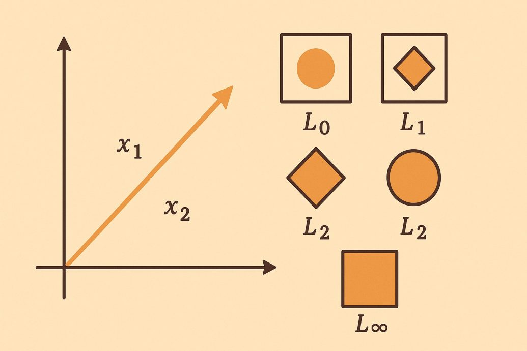
Pictures make this whole idea concrete far faster than raw algebra ever will. The set of vectors whose norm equals one forms a shape called the unit ball. Under the L2 norm that shape is a round circle or a smooth sphere. Under L1 it sharpens into a diamond, and under L-infinity it squares off into a box. Those shapes quietly decide which solutions an optimizer drifts toward in real problems.

These shapes are not merely teaching aids for a tidy textbook diagram. They predict, with surprising accuracy, where an optimizer will place its final answer. A penalty shaped like a diamond rewards solutions that hug the coordinate axes tightly. A penalty shaped like a circle rewards solutions that stay smooth and rounded. Carrying this picture forward turns the upcoming formulas into familiar, friendly landmarks.

The L0 Norm: Counting What Actually Matters

The L0 norm is the eccentric of the family, because it is not really a norm. It simply counts how many components of a vector are different from zero. A vector with three live features and ninety zeros carries an L0 value of three. That blunt tally is exactly what you want when sparsity itself is the goal. It surfaces whenever an engineer wants the smallest possible set of active inputs.

The L0 count breaks the scaling rule, so mathematicians label it a pseudo-norm instead. Doubling a vector leaves its number of nonzero entries completely unchanged. That technicality bothers theorists more than the engineers who prize its bluntness. Minimizing it head-on is brutal, since the problem is combinatorial and not differentiable. No smooth gradient points an optimizer toward a model with fewer active terms.

Because the direct version is intractable, the field reaches for a friendlier substitute. Picking the single best label, for instance, connects to argmax in machine learning routines. The convex stand-in for L0 is the L1 norm, which still drives weights to exact zero. Understanding the L0 wish makes the popularity of L1 feel almost inevitable. That bridge from a sparsity dream to a solvable problem is the heart of this section.

The L1 Norm: Taxicab Distance and Sparsity

Building on that sparsity wish, the L1 norm just sums the absolute value of every component. For the vector three, negative four, zero, the L1 norm comes out to exactly seven. It earns the name Manhattan norm because it measures travel along a grid of streets. The taxicab geometry of city blocks captures that block-by-block intuition perfectly. Among the four measures, L1 is the workhorse of sparse and interpretable modeling.

The diamond shape of the L1 unit ball is precisely why L1 produces exact zeros. Its sharp corners sit right on the axes, where one or more coordinates vanish entirely. Optimizers tend to settle on those corners instead of on the smooth diamond edges. That geometric quirk turns L1 into a quiet, automatic feature selector. Compact models built on multinomial logistic regression often lean on this exact behavior.

L1 also tolerates outliers far better than its squared sibling does. Because it grows only in a straight line, one giant error never swamps the total. That calmness makes it a sensible loss function for noisy, real-world measurements. Practitioners trade this robustness against the harder, non-smooth optimization L1 brings along. The reward is a model that stays steady even when a few readings go haywire.

The L2 Norm: Everyday Euclidean Length

Turning to the most familiar measure, the L2 norm is plain straight-line distance. It squares every component, adds those squares, and takes the square root of the sum. For the small vector three, four, the L2 norm lands on five, the famous triangle answer. This is the very length our eyes, rulers, and tape measures rely on daily. It is also the silent default norm tucked inside countless machine learning routines.

Squaring makes the L2 norm punish large components far more sharply than small ones. A single component of size ten already contributes one hundred before the root. That pressure nudges optimizers to spread magnitude evenly over many tiny weights. The outcome is the smooth, balanced weight pattern that L2 regularization is known for. The same averaging instinct shows up in how batch normalization speeds up networks.

The L2 norm is smooth at every point, which makes gradient descent genuinely happy. Its derivative stays simple, continuous, and stable across the whole parameter space. That smoothness is why squared penalties appear in ridge regression and weight decay. Optimizers such as the Adam optimizer in machine learning mesh cleanly with L2 terms. Few measures pair such smoothness with such immediate geometric meaning.

Euclidean length also gives clean meaning to similarity, projection, and angle. Cosine similarity, for one, divides a dot product by two separate L2 norms. Clustering and nearest-neighbor search usually measure closeness with this same trusted length. Among the four measures, L2 is the one tied most tightly to intuition. That intuition is why newcomers nearly always meet this norm before any other.

The L-Infinity Norm: When Only the Worst Case Counts

Beyond the everyday cases sits the L-infinity norm, also called the maximum norm. It reports the single biggest absolute value across all components and ignores the rest. For the vector three, negative four, zero, the L-infinity norm equals exactly four. The name comes from letting the exponent p grow without limit in the Lp formula. As p climbs, the largest term quickly drowns out every smaller contribution.

The L-infinity unit ball is a square or cube whose flat faces align to the axes. A constraint in this norm caps every coordinate by the very same fixed amount. That makes it the natural language for per-feature budgets and strict worst-case limits. Robustness researchers use it to bound how far an input may safely be nudged. It asks a sharply different question than the averaging L1 and L2 measures do.

Because it watches only the extreme, L-infinity reacts to a single spike. One outsized component changes the value while every other entry stays irrelevant. That focus is a gift for safety analysis and a nuisance for smooth fitting. Sequence models such as long short-term memory networks sometimes bound activations this way. Engineers pick it when the worst case matters more than the average.

L1 Versus L2: The Difference That Shapes Models

Shifting to the question readers ask most, the L1 and L2 gap is sparsity against smoothness. L1 forces many weights to exactly zero and keeps only a handful of strong ones. L2 keeps every weight alive but holds each one small and well balanced. The difference between the L1 and L2 norm is really a choice about model shape. That choice then echoes through interpretability, stability, and raw storage cost.

Reach for L1 when you want a short, explainable shortlist of important features. Sparse models load faster, audit more easily, and shrug off several forms of overfitting. They fit genomics, text, and any setting with thousands of candidate input variables. The catch is tougher optimization and wobble when input features correlate strongly. Many teams sanity-check such models against the theory behind machine learning.

Reach for L2 when you want stable predictions and smooth, well-mannered gradients. Ridge penalties shine when many features each carry a small slice of real signal. They treat correlated inputs gracefully instead of dropping one of a pair at random. The price is a dense model that resists tidy human explanation afterward. Most deep networks default to L2 weight decay for exactly these reasons.

Plenty of pipelines simply blend both penalties in a method called the elastic net. The mixture keeps some sparsity from L1 and some welcome stability from L2. Tuning that balance is a routine hyperparameter search, not a dark art. This compromise shows the measures behave as teammates rather than as rivals. You rarely need to crown a single permanent winner among the vector norms.

Reading the Unit Balls: A Visual Mental Model

Beyond the formulas, sketching the unit balls is the fastest way to feel the difference. The L1 diamond, the L2 circle, and the L-infinity square nest neatly inside one another. The diamond fits within the circle, and the circle fits snugly within the square. That nesting mirrors a very real inequality among the three measures on any fixed vector. Models like radial basis function networks rely heavily on this distance geometry.

For any vector, its L-infinity value stays below its L2 value, which stays below its L1 value. That ordering explains why a sparse corner solution looks so unlike a smooth one. An L1 constraint tugs the answer toward the diamond corners that sit on the axes. The same problem under L2 settles on a rounded point holding no exact zeros. Seeing the shapes makes the underlying algebra feel inevitable rather than mysterious.

This nesting also hints at why converting between norms is sometimes genuinely useful. A bound proved in one norm can be loosened or tightened into another. Engineers exploit that freedom when one norm is easier to compute than another. The shapes, in other words, are a practical tool and not mere decoration. Keeping all three in mind makes the later sections about duality far easier. That payoff alone makes the small effort of sketching them worthwhile. A quick drawing on paper often clarifies more than a page of dense formulas. Many engineers keep these three shapes pinned mentally for fast reasoning.

Vector Norms and the Triangle Inequality

Beyond size alone, every genuine norm must respect the triangle inequality. That rule says the norm of a sum never exceeds the sum of the norms. In plain words, a detour through a third point can never beat going direct. This single property is what makes vector norms behave like sensible distances. Without it, the whole geometry of optimization would quietly fall apart.

The triangle inequality is the quiet axiom that lets norms define trustworthy distances. It guarantees that nearby vectors stay nearby after small, reasonable changes. The triangle inequality holds for the L1, L2, and L-infinity norms alike. That shared property is exactly why all three qualify as genuine norms. The L0 count fails it, which is one more reason it stays a pseudo-norm.

This axiom also underpins convergence proofs across optimization and analysis. Many guarantees bound an error by the norm of a difference of vectors. The inequality then chains those bounds together into a clean final result. Strip the rule away and most of those careful proofs simply collapse. So a humble fact about detours quietly supports a great deal of theory.

Practitioners rarely invoke the inequality by name during everyday work. Yet it silently justifies treating a norm as a measure of real distance. Every clustering run and nearest-neighbor lookup leans on that quiet justification. The rule also explains why mixing incompatible metrics produces nonsense results. Respecting it keeps a pipeline mathematically honest from end to end.

Seen this way, the triangle inequality ties the whole family together neatly. It is the shared contract that L1, L2, and L-infinity all sign. That contract is what lets us compare these vector norms on equal footing. It also marks the precise line that the blunt L0 count refuses to cross. Holding that boundary in mind sharpens every later choice among the measures.

Dual Norms and the Hidden Symmetry

Stepping back to a deeper layer, every norm carries a partner called its dual norm. The dual measures the largest projection a unit vector can make against a fixed target. A celebrated result says the dual of the L-infinity norm is the L1 norm exactly. The pairing even works both ways, so L1 and L-infinity are duals of each other. This tidy relationship surfaces again and again across optimization and analysis.

The L2 norm is unusual because it is its own dual, a trait called self-duality. That clean symmetry is one reason Euclidean geometry feels so balanced and friendly. Duality also explains why a constraint in one norm maps to a penalty in another. It links robustness budgets written in L-infinity to sparse goals written in L1. Such ideas appear in signal work like the frequency domain in AI.

Dual norms are far more than decorative trivia for optimization theorists. They quietly power the bounds that prove a model resists a whole family of attacks. They also set the step rules inside many modern optimization algorithms. Knowing the duals turns a flat list of measures into a connected, navigable map. That map lets researchers move with confidence between robustness and sparsity goals. Even simple gradient methods quietly rely on a dual norm to size each step. The theory may look abstract, yet it shapes very practical training choices daily. That hidden link is why a curious engineer benefits from learning it once.

Turning Vectors Into Unit Length

Among the everyday chores norms handle, rescaling a vector to unit length stands out. Dividing a vector by its L2 norm yields a unit vector pointing the same direction. That step, called normalization, keeps direction while discarding the raw magnitude. Many algorithms care only about direction, so the trick appears constantly in practice. Normalizing early often stabilizes training and makes features comparable across wildly different scales.

L2 normalization is the quiet step behind cosine similarity and most modern embeddings. Once vectors share unit length, their dot product becomes the cosine of their angle. That keeps comparisons fair, since long vectors no longer win on scale alone. Search and clustering systems lean on this convenient property every single day. Forgetting to normalize is a classic source of silently biased similarity scores.

You can also normalize with other vector norms when a task asks for it. Dividing by the L1 norm forces the absolute components to sum to one. That move turns a vector into something close to a probability-style weighting. Dividing by the L-infinity norm instead caps the single largest component at one. Each variant reshapes the vector differently, so the goal should pick the norm.

One sharp edge is that the zero vector cannot be normalized at all. Its norm is zero, and dividing by zero stays undefined in every library. A tiny epsilon added to the denominator is the standard defensive patch. This little detail still trips up many implementations during early development. Handling it upfront saves hours of baffling debugging later in a project.

Norms Inside Loss Functions: MAE Versus MSE

On top of regularization, vector norms quietly define the loss functions models minimize. Mean absolute error sums the L1 distances between predictions and their true targets. Mean squared error squares those errors instead, which is an L2-style penalty at heart. The two losses inherit the personalities of the L1 and L2 norms directly. Choosing between them is really a choice about how to treat large mistakes.

Mean squared error punishes big errors quadratically, so a few large misses dominate it. That sensitivity to outliers mirrors the behavior of the L2 norm exactly. Mean absolute error grows only linearly, so it stays calm when outliers appear. The scikit-learn metrics guide lays out both losses and their typical uses. Picking the wrong loss can bias a model toward or away from rare extremes.

The smoothness gap also surfaces while optimizing these two losses. Squared error has a smooth gradient everywhere, which gradient descent handles with ease. Absolute error has a kink at zero, which can slow or complicate convergence. Engineers often blend the two into a Huber loss to grab both benefits. That hybrid acts like squared error near zero and like absolute error far away.

Computing Norms With NumPy and PyTorch

In practice, you rarely compute vector norms by hand past the toy stage. NumPy exposes them through one function that accepts an order argument directly. Passing one, two, or infinity picks the L1, L2, or L-infinity norm cleanly. The same pattern repeats across deep learning frameworks with almost identical names. That uniform interface makes switching norms a one-line edit in most code.

PyTorch copies this design and computes vector norms on tensors sitting on a GPU. Its linear algebra module follows the same order convention NumPy set years earlier. The PyTorch norm documentation spells out every order and dimension argument carefully. Choosing the wrong axis is the most common blunder when norms hit batched tensors. Reading the shape rules once heads off a whole class of silent bugs.

Performance starts to matter once vectors swell into millions of dimensions. Library routines use tuned linear algebra kernels that beat naive Python loops handily. They also guard numerical stability better than a quick hand-rolled square and root. On very large models, even a norm can appear on a profiler’s hot list. Trusting the library is almost always the faster and safer call.

From Vectors to Matrices: Matrix Norms

From there, the same magnitude idea climbs naturally from vectors up to matrices. A matrix norm measures the size of a matrix with one non-negative number. The Frobenius norm treats the matrix as one long vector and takes its L2 norm. Spectral and nuclear norms instead measure how much a matrix can stretch a vector. These matrix norms build straight on the vector norms covered earlier here.

The spectral norm equals the largest singular value and bounds how far a matrix stretches input. That property puts it at the center of stability analysis in deep networks. Researchers constrain it to stop layers from amplifying their signals out of control. The matrix norm reference lists the common families and their formulas. Each family asks a different question about a matrix, much as vector norms do.

Spectral normalization has grown into a popular trick for steadying generative models. It rescales each weight matrix so its spectral norm stays near one. That keeps gradients tame and curbs the oscillations that wrecked early training runs. The cost is extra work to estimate the largest singular value each step. Teams accept the overhead because the stability payoff is usually well worth it.

The nuclear norm, the sum of singular values, pushes toward low-rank solutions. It plays the sparsity-promoting role for matrices that L1 plays for plain vectors. Recommender systems use it to complete sparse rating tables from partial data. The drawback is that computing it needs a full singular value decomposition. That cost still keeps the nuclear norm out of the very largest settings today. Approximate solvers can estimate the leading singular values when speed matters most. Those shortcuts trade a little precision for a large gain in raw throughput. Teams weigh that bargain against the accuracy their specific task truly needs.

The Wider Lp Family: Fractional and Large p

Among the wider Lp family, the values between zero and one are the oddballs. These fractional norms are not convex, so optimizing them directly is genuinely hard. They drive solutions toward sparsity even more fiercely than the familiar L1 norm. Researchers sometimes accept them when extreme sparsity outweighs the optimization pain. The cost is that local minima multiply and clean convergence guarantees mostly vanish.

As the exponent p grows very large, the Lp norm steadily approaches the L-infinity norm. The biggest component dominates the sum more and more as p keeps climbing. By the time p reaches a few hundred, the result barely differs from the maximum. That limit is exactly why the maximum norm wears the infinity label. Seeing the continuum makes the named norms feel like landmarks on a single dial.

Choosing an exotic p is rare but occasionally pays off on niche problems. Robust statistics sometimes favors a value slightly above one to balance outliers. Signal processing experiments with fractional norms to recover extremely sparse signals. Most production systems still stick to one, two, or infinity for good reason. Those three values cover the vast majority of practical machine learning needs.

Norms Powering Search and Recommendation

Turning to large systems, vector norms quietly run modern search and recommendation. Documents, products, and users all become dense embedding vectors in such systems. Finding relevant items means measuring distance or similarity between those vectors fast. The chosen norm decides which items count as near and which count as far. That single decision shapes the quality of results real users finally see.

Most retrieval stacks normalize embeddings and then rank by cosine similarity under L2. Normalization strips length effects so that only direction drives the final ranking. Approximate nearest-neighbor indexes then sweep billions of vectors in milliseconds. These indexes assume one norm, so a mismatched metric quietly degrades the output. Matching the index metric to the training metric is easy to overlook.

Some systems favor the L1 norm when features are counts or sparse histograms. Manhattan distance can behave more sensibly than Euclidean distance in high dimensions. A known curse is that distances concentrate as dimensionality climbs into the thousands. That effect blurs the gap between near and far neighbors under any norm. Engineers fight back with dimensionality reduction and carefully trained embedding spaces.

Recommendation quality therefore rides on more than a clever model alone. The metric, the normalization step, and the index all interact in subtle ways. A mismatch among them can erase the gains from a better model entirely. Careful evaluation across the whole pipeline is the only dependable safeguard. Norms sit quietly at the center of that pipeline the entire time. A careful audit of the metric often recovers more quality than a bigger model. Small mismatches compound quietly until they noticeably blunt the final results. Fixing them early is usually the cheapest reliable win available to a team.

Why L2 Rules Weight Decay

Given how smooth the L2 norm is, it became the default regularizer in deep learning. Weight decay adds a small fraction of the squared L2 norm to the training loss. That term gently tugs every weight toward zero on each optimization step. The pull stops any single weight from ballooning and dominating the model. Smaller weights tend to generalize better and resist overfitting on thin data.

Weight decay and the L2 penalty are close cousins, though not identical in modern optimizers. With plain gradient descent the two formulations line up almost exactly. With adaptive methods the decoupled version usually behaves noticeably better. That subtle distinction surprised many practitioners when it was first documented clearly. Knowing which variant your framework uses prevents quietly inconsistent results.

The strength of weight decay is a hyperparameter that rewards careful tuning. Too little leaves the model free to overfit the training data badly. Too much shrinks the weights until the model underfits almost everything. A short sweep over a few values usually finds a sensible range fast. Documenting the winning value also helps the next engineer reproduce the result.

Comparing the Four Norms at a Glance

For teams deciding fast, one compact table often settles the debate quicker than theory. The grid below lines the four measures up across the properties engineers weigh most. It spans the formula idea, geometry, sparsity, outlier behavior, smoothness, and typical use. Reading across a row shows why a measure fits a job, and down a column shows the trade. A single careful glance can replace a long, inconclusive argument at the whiteboard.

Treat the table as a launch point, then confirm the pick with a quick validation run. No measure wins every contest, and the surrounding context always decides the answer. Most teams test two candidate norms and compare validation scores before committing. The pitfalls row deserves a careful second read before any design is locked. Treating the grid as a hypothesis rather than a verdict keeps the whole decision honest.

Property	L0	L1	L2	L-infinity
Formula idea	Count nonzeros	Sum absolutes	Root of squares	Max absolute
Unit ball shape	Discrete	Diamond	Circle	Square
Sparsity	Exact target	Strong	None	None
Outlier sensitivity	Low	Low	High	Highest
Smoothness	None	Partial	Full	Partial
Differentiable	No	Almost	Yes	Almost
Typical use	Feature counting	Sparse models	Weight decay	Robustness bounds
Common pitfall	Intractable	Unstable ties	Dense weights	Spike sensitive

Putting Norms to Work Across a Pipeline

Moving on to daily practice, vector norms turn up at nearly every stage of a model. They define loss functions, regularizers, gradient clipping rules, and similarity scores. Most libraries expose them through one tidy call like the NumPy linear algebra module. The NumPy norm documentation switches among L1, L2, and L-infinity with one argument. That convenience hides a real decision that still deserves genuine thought.

Regularization is the most common spot where a norm rewrites a model’s whole personality. An L1 penalty shrinks weights toward zero and trims redundant features automatically. An L2 penalty keeps every weight alive but holds them small and steady. The penalty strength is a hyperparameter you tune against held-out validation data. Getting it wrong underfits or overfits no matter how strong the architecture.

Gradient clipping is a second everyday use that keeps training from blowing up. Engineers cap the L2 norm of the gradient at a fixed threshold each step. That trick steadies deep and recurrent models that would otherwise diverge mid-run. It is standard when training recurrent neural networks explained elsewhere here. Without it, one bad batch can erase hours of careful progress.

Distance and similarity round out the list of routine applications. Nearest-neighbor search, clustering, and retrieval all rest on one chosen measure. Swapping L2 for L1 can change which neighbors a system calls the closest. The right pick depends on the data, the task, and the cost of errors. That is why careful engineers never treat the choice as a throwaway default.

Risks and Where Norm Penalties Fall Short

Despite their reach, these measures cure only some modeling problems, not all. A penalty can shrink the wrong weights when features sit on mismatched scales. Standardizing inputs first is required, or the norm favors large-scale features unfairly. That preprocessing step is easy to skip and painful to debug much later. Everyday systems in examples of AI in everyday life all depend on this hygiene.

Sparse L1 solutions turn unstable when several features carry nearly identical signal. The method may keep one feature and drop its near-twin almost at random. Small data shifts then flip which feature survives, which corrodes user trust. L2 or the elastic net usually calms this at a cost in interpretability. No penalty, though, can erase the underlying ambiguity hiding in the data.

Norms also assume that magnitude is the one quantity worth controlling. Some problems care far more about ordering, structure, or fairness than raw size. In those cases a plain penalty can optimize the wrong objective without warning. Recognizing this limit keeps these measures in their proper supporting role. They make powerful servants but genuinely poor masters of an objective.

The Ethics of Trimming Models With Norms

Looking ahead to responsibility, the choice of norm carries quiet ethical weight in deployment. A sparse model that drops a feature may discard signal that protected a small group. The math looks neutral, yet the dropped feature can encode a fairness-relevant pattern. Audits must ask who gains and who loses when a penalty trims the model. The cost of skipping that review usually lands on the least visible users.

Interpretability from L1 can mislead if stakeholders read sparsity as proof of fairness. A short, clean feature list still hides whatever bias lived in the data. Teams should pair norm-based selection with explicit bias testing across affected subgroups. Recording why each feature stayed or left builds real, durable accountability. Responsible practice treats these measures as one input to ethics review, never the verdict.

The Future of Vector Norms in Deep Learning

Looking ahead, vector norms keep collecting fresh roles as models swell in size. Norm-based gradient clipping is now standard for training huge language models safely. Researchers also study spectral and structured norms that act on whole weight matrices. Those richer measures carry the same magnitude logic from vectors up to layers. The core intuition behind the classic norms still anchors each new variant.

Robustness research is pushing L-infinity bounds steadily into mainstream safety certification. Provable guarantees increasingly state how far an input may move under that norm. As regulation tightens, those worst-case measures will likely become routine reporting. Compression and on-device models keep sparsity, and therefore L1, in steady demand. New architectures like neural architecture search still tune these penalties.

The long arc points toward measures tailored to specific structures and tasks. Graph, sequence, and image models each invite a norm that respects their shape. Generative systems like generative adversarial networks already use specialized penalty terms. None of that replaces the four classics this guide has carefully covered. Mastering them stays the fastest route into every advanced variant ahead. Each fresh variant still reduces, at its core, to measuring magnitude wisely. That continuity is exactly why the fundamentals reward a patient, careful study. Engineers who learn the basics deeply adapt to new measures with little friction.

Vector Norms in the Wild: Worked Examples

Real systems show how these measures earn their keep beyond the textbook. Each example below ties a concrete method to the norm that makes it work. The cases span genomics, medical imaging, and the security of deployed models.

Lasso Regression for Gene Selection

The lasso, introduced by Robert Tibshirani in 1996, used an L1 penalty to select a few predictive genes. Genomic datasets routinely hold more than 20,000 candidate genes, yet only a few dozen drive a disease. The L1 term drives most coefficients to exactly zero, often removing more than 95 percent of inputs. Researchers built diagnostic gene panels on these sparse fits and reported far easier clinical interpretation. The documented limit is instability, since correlated genes still make the method keep one and drop a near-duplicate. The history of the lasso estimator records how this L1 idea reshaped statistics.

Compressed Sensing for Faster MRI

Compressed sensing MRI, pioneered by Michael Lustig and colleagues around 2007, used L1 minimization to rebuild images. The method adopted sparsity in a transform domain and reduced the data collected by roughly 5 times. That reduction produced scans that ran in a fraction of the usual minutes, easing patient discomfort. Hospitals piloted these reconstructions and produced diagnostic images from heavily undersampled raw measurements. The known trade is that aggressive undersampling still risks subtle artifacts that demand careful tuning and expert review. A widely cited compressed sensing summary documents this L1-driven breakthrough.

L-Infinity Budgets for Adversarial Robustness

Adversarial robustness research adopted the L-infinity norm to define how far an attacker may nudge each pixel. A standard benchmark caps the perturbation at 8 divided by 255 on image datasets such as CIFAR-10. Defenders trained models against this exact budget and produced a measurable increase in certified accuracy. The approach built provable guarantees that hold for every input inside the L-infinity ball around a sample. The persistent limit is that robustness within one budget still leaves gaps under other threat models. The adversarial training paper by Madry and colleagues formalized this L-infinity threat model.

Lessons From Production Norm-Driven Systems

Production stories expose trade-offs that tidy formulas tend to hide. These cases show the measures shaping cost, speed, and stability at real scale. Each one names the problem, the chosen fix, and the catch that lingered.

Case Study: Ridge Regression Steadying Risk Scores

A lending team faced wild coefficient swings because dozens of credit features were strongly correlated. They built an L2 ridge penalty into the model, which needed only one new hyperparameter to tune. The squared norm spread weight across correlated inputs instead of dropping features at random each retrain. Score volatility fell sharply, cutting month-to-month variance by double-digit percent across 40 input features. The limit they accepted is that the dense L2 model still resists simple explanation to regulators. Guidance in the Keras loss functions guide covers how such penalties enter training.

Case Study: L1 Pruning for On-Device Vision

A mobile team needed a vision model that still ran fast on a low-power phone chip. They adopted L1-based weight pruning, which trained the network to push small weights toward zero. The sparse result let them remove roughly 60 percent of parameters with only minor accuracy loss. Inference latency dropped by several milliseconds per frame, which mattered for a real-time camera feature. The required catch is that extreme pruning still degrades accuracy unless retraining recovers the lost capacity. Background on efficient training appears in how data augmentation works for vision.

Case Study: Gradient Clipping in Language Model Training

A research group training a large language model kept hitting loss spikes that ruined long runs. They ran gradient clipping that capped the global L2 norm of the gradient near a threshold of 1.0. This one rule rescaled any oversized update before it could destabilize the network weights. Training became reliably stable, and the team saved many hours of wasted compute on failed restarts. The trade is that clipping still adds a hyperparameter that must be tuned for each new setup. The technique traces to the gradient clipping paper by Pascanu and colleagues.

Key Insights

• The lasso introduced L1 penalties in 1996 and now selects a few genes from over 20,000 candidates routinely.
• Compressed sensing used L1 minimization to cut MRI sampling by roughly 5 times while preserving diagnostic image quality.
• Adversarial defenses adopt an L-infinity budget of 8 divided by 255 to certify robustness on standard image benchmarks.
• Gradient clipping caps the L2 gradient norm near 1.0 and stabilizes the training of very deep networks.
• The L2 norm is self-dual, while the L1 and L-infinity norms are duals of each other in optimization.
• On any vector, the standard norm inequalities keep the L-infinity value below the L2 value below the L1 value.
• Standard libraries such as NumPy linear algebra switch among L1, L2, and L-infinity with one argument.

Taken together, these facts show that vector norms are practical levers, not abstract symbols. Each measure encodes a different belief about what magnitude should mean for a task. Sparsity, smoothness, and worst-case control are the three goals these measures serve. The right pick flows from the data, the cost of errors, and the need to explain results. Mastering this small family pays off across regression, deep learning, and serious model safety.

Common Questions About Vector Norms