
Introduction: Project Description
Cricket is a strategic game that unfolds on a field between two teams of eleven players each, aiming to outscore each other. It’s the strategy, the uncertainty of outcomes, and the beauty of teamwork that make cricket a rich ground for data analysis and predictive modeling.
With Python as our primary tool, this guide will walk you through the intriguing world of data analysis and predictive modeling applied to the Indian Premier League (IPL) – the crown jewel of cricketing events. We will dive deep into match statistics and team performances, uncovering hidden patterns and trends. We will craft features, and design models, and put them to test.
Table of contents
- Introduction: Project Description
- Problem Statement: Understanding the Cricketing Framework
- Data Collection
- Exploratory Data Analysis (EDA)
- Correlation Matrix
- Data Preprocessing
- Data Preparation: Establishing Features and Target Variable
- Label Encoding
- Train/Test Split and Feature Scaling
- Model Building: Random Forest Classifier
- Model Training and Evaluation
- Feature Importance
- What have we learned?
- Conclusion
- References
Problem Statement: Understanding the Cricketing Framework
Before delving into the data-driven aspects of the game, it’s essential to understand its framework. Cricket unfolds on a rectangular 22-yard pitch set in the center of an oval field. Two wickets, each a set of three wooden stumps topped by two bails, mark either end of the pitch.
The teams alternate between batting and fielding roles across different phases known as innings. The objective of the batting team is to amass as many runs as possible. At the same time, the fielding team endeavors to limit these runs, primarily through bowling strategies and field placements. The usual flow involves the teams switching roles post-inning.
The match’s format defines the number of innings. The traditional Test match, the lengthiest format of the game, generally includes two innings for each team. In contrast, shorter versions like One Day International (ODI) and Twenty20 (T20), common in the IPL, feature one inning per team. The team that garners the highest sum of runs across all innings is declared the winner.
We will start from scratch, embarking on the journey of data acquisition, wrangling, and preprocessing, diving into exploratory data analysis, followed by feature selection and engineering. Finally, we will leverage machine learning models to predict future match outcomes. The content is detailed, thorough, and well-documented, providing an in-depth understanding and practical application of predictive modeling in sports.
Data Collection
Our predictive modeling journey starts with data acquisition. The data used in this project is IPL data obtained from Cricsheet, a prominent online resource providing comprehensive datasets for cricket matches. The datasets we utilize encompass detailed information about IPL matches and individual ball-by-ball data. These datasets are loaded into pandas DataFrames named ‘matches’ and ‘deliveries’ for match level and delivery (ball-by-ball) level data respectively.
For the scope of this project, we will solely focus on the IPL data spanning from 2008 to 2017. It is during this ten-year period that we aim to unravel patterns and predictions, providing a comprehensive yet focused analysis.
We will use various Python libraries for data processing and analysis such as NumPy, pandas, seaborn, and matplotlib, as well as the sci-kit learn library for machine learning tasks. The libraries have been imported at the top of the script.
import pandas as pd

matches = pd.read_csv('matches.csv')
deliveries = pd.read_csv('deliveries.csv')

Exploratory Data Analysis (EDA)
We kick-start our analysis by loading the necessary libraries and the IPL dataset. Subsequently, we’ll engage in exploratory data analysis, identifying key patterns and insights through visualizations. We’ll also develop a machine learning model to predict match outcomes. Ensure that you adjust the file paths according to your data location:
We’ll begin by loading the necessary libraries and the IPL dataset. Afterwards, we’ll perform exploratory data analysis and visualizations to identify key patterns and interesting insights. We’ll also prepare a machine-learning model for predicting the outcome of the matches.
Most successful teams: Looking at the vibrant bar graph, one can’t miss that Mumbai Indians stand tall, emerging as the most successful team with a whopping 92 victories under their belt. It’s followed by Chennai Super Kings, Kolkata Knight Riders, Royal Challengers Bangalore, and Kings XI Punjab. These are the juggernauts of the game, and it would be interesting to see how this dominance affects their performance in upcoming seasons.
Venues that hosted the most number of matches: Cricket is not just about the teams, but also where they play. The M Chinnaswamy Stadium emerges as the most favored cricket venue, hosting 66 matches, followed closely by the iconic Eden Gardens and the historical Feroz Shah Kotla. Venues can play a significant role in matches due to factors such as pitch behavior, stadium size, and crowd support. This information could be pivotal in predicting future match outcomes.
Toss decisions across seasons: The toss is a crucial element of cricket strategy. Interestingly, teams’ preferences for batting or fielding after winning the toss seem to vary across seasons. Understanding these preferences could give us insight into the teams’ strategies and possibly their performance in different conditions.
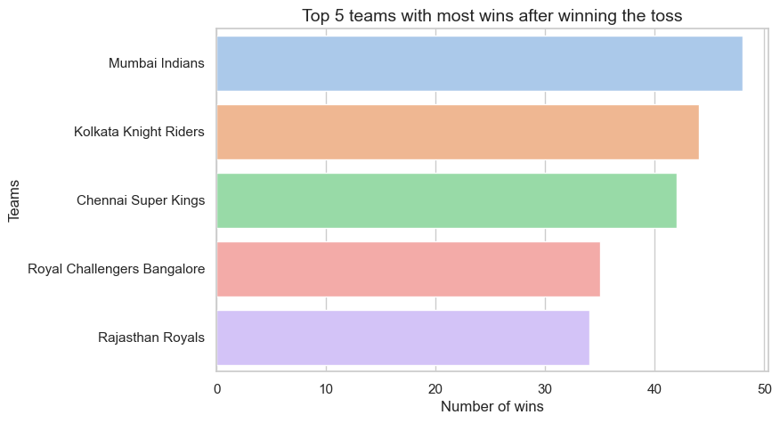
Team Performance after winning the toss: Winning the toss doesn’t always mean winning the match, but Mumbai Indians again top the chart, translating their toss wins into overall victories 48 times. It’s important to note that while winning a toss can give teams an initial advantage, it’s ultimately their performance that determines the match outcome.
Top umpires who officiated most matches: Umpires are an integral part of the sport. The graph shows us that HDPK Dharmasena has officiated the most matches, followed by S Ravi, AK Chaudhary, C Shamshuddin, and SJA Taufel. This could hint at their experience and credibility in the field.
import matplotlib.pyplot as plt
import seaborn as sns


sns.set(style="whitegrid")
sns.set_palette("pastel")

# Assuming 'matches' dataframe is already loaded with data

# 1. Most successful teams
teams = matches['winner'].value_counts().head(5)
plt.figure(figsize=(8,5))
sns.barplot(x=teams.values, y=teams.index, palette="pastel")
plt.title('Top 5 most successful teams', fontsize=14)
plt.xlabel('Number of matches won', fontsize=12)
plt.ylabel('Teams', fontsize=12)
plt.show()

# 2. Venues that hosted most number of matches
venues = matches['venue'].value_counts().head(5)
plt.figure(figsize=(8,5))
sns.barplot(y=venues.index, x=venues.values, palette="pastel", orient='h')
plt.title('Top 5 venues that hosted most matches', fontsize=14)
plt.xlabel('Number of matches', fontsize=12)
plt.ylabel('Venues', fontsize=12)
plt.show()


# 3. Toss decisions across seasons
plt.figure(figsize=(8,5))
sns.countplot(x='season', hue='toss_decision', data=matches, palette="pastel")
plt.title('Toss decisions across seasons', fontsize=14)
plt.xlabel('Season', fontsize=12)
plt.ylabel('Count', fontsize=12)
plt.show()

# 4. Team Performance after winning the toss
toss_wins = matches[matches['toss_winner'] == matches['winner']]['winner'].value_counts().head(5)
plt.figure(figsize=(8,5))
sns.barplot(x=toss_wins.values, y=toss_wins.index, palette="pastel")
plt.title('Top 5 teams with most wins after winning the toss', fontsize=14)
plt.xlabel('Number of wins', fontsize=12)
plt.ylabel('Teams', fontsize=12)
plt.show()

# 5. Top umpires who officiated most matches
umpires = pd.concat([matches['umpire1'], matches['umpire2']]).value_counts().head(5)
plt.figure(figsize=(8,5))
sns.barplot(y=umpires.index, x=umpires.values, palette="pastel", orient='h')
plt.title('Top 5 umpires officiating most matches', fontsize=14)
plt.xlabel('Number of matches', fontsize=12)
plt.ylabel('Umpires', fontsize=12)
plt.show()


Match Outcome vs Toss Winning Team: The pie chart provides an intriguing look at the correlation between winning the toss and winning the match. Contrary to what many might think, the pie chart reveals that the toss only results in a victory 51.4% of the time, proving that cricket is indeed a game of uncertainties.
# Determine outcomes
victory_with_toss = matches[(matches.result == 'normal') & (matches.toss_winner == matches.winner)].id.count()
defeat_with_toss = matches[(matches.result == 'normal') & (matches.toss_winner != matches.winner)].id.count()

outcome_data = pd.DataFrame({
'Match Outcome': ['Victory', 'Defeat'],
'Toss Winning Team': [victory_with_toss, defeat_with_toss]
})

plt.style.use('seaborn-pastel')

# Produce a pie chart
fig, ax1 = plt.subplots()
ax1.pie(outcome_data['Toss Winning Team'], labels=outcome_data['Match Outcome'], autopct='%1.1f%%', startangle=90, colors=['lightblue', 'lightcoral'])

ax1.axis('equal')
plt.title('Match Outcome vs Toss Winning Team')
plt.show()
These fascinating findings give us rich insights into the sport. It’s not just about the players or teams, but also about the strategy, venue, toss decisions, and even the umpires. Using this information could make future match predictions more precise.
Correlation Matrix
In the Correlation matrix, every cell is characterized by a value known as the Pearson correlation coefficient, or simply, the correlation coefficient. This coefficient quantifies the degree and direction of the linear relationship between paired variables. It ranges from -1 to 1, where:
-1 implies a perfectly inverse or negative linear correlation
0 indicates an absence of linear correlation
1 signifies a perfect positive linear correlation
# Discard unnecessary columns from the dataframe.
matches.drop(columns=['player_of_match', 'dl_applied', 'result', 'umpire1', 'umpire2', 'date', 'season', 'id'], inplace=True)

# Clean the dataset by removing rows with missing 'winner' data.
matches = matches[matches['winner'].notna()]

# Set the data types of categorical variables.
categorical_vars = ['team1', 'team2', 'winner', 'venue', 'toss_winner', 'toss_decision']
for var in categorical_vars:
matches[var] = matches[var].astype('category')

# Apply label encoding to the categorical variables.
for var in categorical_vars:
matches[var] = matches[var].cat.codes

# Display the first few rows of the dataset after conversion.
matches.head()

# Begin constructing a correlation matrix.
import numpy as np

# Compute pairwise correlation of columns.
correlation_data = matches.corr()

# Generate a mask for the upper triangle.
upper_triangle_mask = np.triu(np.ones_like(correlation_data, dtype=bool))

plt.figure(figsize=(10,8))
color_map = sns.diverging_palette(220, 10, as_cmap=True)

# Create a heatmap with the provided data, mask, and color map.
sns.heatmap(correlation_data, mask=upper_triangle_mask, cmap=color_map, center=0, annot=True, fmt=".2f",
square=True, linewidths=.5, cbar_kws={"shrink": .5})


plt.title('Correlation Matrix for Variables')
plt.show()
The team1, team2, toss_winner, and winner columns have relatively high correlations. This suggests that the team that wins the toss is more likely to win the match. This could be due to the advantages of choosing whether to bat or field first based on the conditions of the pitch and weather.
The toss_decision column, however, shows a low correlation with the winner, suggesting that the decision made after winning the toss (whether to bat or field) doesn’t seem to have a significant impact on the outcome of the match. This is somewhat counter-intuitive as it’s generally believed that the decision to bat or field first can influence the game’s result. But in this dataset, the statistical evidence does not support that belief.
The win_by_runs and win_by_wickets columns show a strong negative correlation. This is expected because if a team wins by a high number of runs, it means they defended their score well and didn’t let the other team reach it, thus they won’t have many wickets to take. Similarly, if a team wins by a high number of wickets, it means they reached the target score easily, thus they won’t have many runs to defend.

Now that we’ve established a firm grip on our data, let’s pivot toward the actual predictive modeling. The road to meaningful predictions is paved with necessary data transformations, model selection, hyperparameter tuning, and performance evaluation.
Data Preprocessing
The journey begins with preprocessing our data. Here, we substitute missing player dismissal instances with a ‘0’ via the fillna() function. This ensures that our model doesn’t stumble upon undefined data during training, which might lead to inaccurate predictions.
Further, to standardize our data, we replace all non-zero instances of player dismissals with ‘1’, indicating a dismissal occurrence. In effect, we create a new binary feature – ‘player_dismissed’ – where ‘1’ denotes a dismissal and ‘0’ stands for the lack thereof.
Data Preparation: Establishing Features and Target Variable
The following stage involves structuring our dataset by creating features that would play a vital role in determining the outcome of a match. We created two features – ‘run_total‘ and ‘dismissed_players‘ – by converting the corresponding columns into numeric data types.
Next, we used groupby and aggregation functions to create a comprehensive match-level dataset. This new dataframe – ‘train_data‘ – consists of match_id, inning, over, team1, team2, batting_team, and winner. It also includes the aggregated sum of ‘run_total‘ and ‘dismissed_players‘ for every unique combination of the above variables.
We then create two cumulative features: ‘wickets_in_innings‘ and ‘score_in_innings‘. The former aggregates the total wickets lost by a team in an inning up until the current over, while the latter calculates the team’s total score in an inning up until the current over.
The next step is defining our independent features (X) and the dependent target variable (y). The features (X) are the variables that influence the outcome we are trying to predict, which is encapsulated by the target (y). For our case, the features include innings, overs, total runs, dismissed players, wickets in innings, score in innings, team1, team2, and batting team. The target is the ‘winner’ of the match.
Label Encoding
To make our categorical data palatable for machine learning algorithms, we employ label encoding. This transforms categorical textual data into a machine-understandable numerical format. Sci-kit Learn’s LabelEncoder aids us in this process.
Train/Test Split and Feature Scaling
Following this, we partition our data into a training set (to train the model) and a testing set (to evaluate the model’s performance). We use 80% of our data for training and reserve 20% for testing. Post-split, we scale our features to a standardized scale using the StandardScaler. This normalization ensures that all features contribute equally to the result, which is especially crucial for algorithms that use distance-based metrics.
Model Building: Random Forest Classifier
Our predictive model of choice here is the Random Forest Classifier. It’s a powerful ensemble learning method that operates by creating a multitude of decision trees at training time and outputting the class that is the mode of the classes or the mean prediction of the individual trees. Its robustness and versatility allow it to handle both classification and regression tasks, and most importantly, it effectively mitigates the issue of overfitting, which is a common pitfall of decision trees.
Each decision tree in the ‘forest’ learns from a different sample of data, contributing to diverse perspectives and ensuring that the model doesn’t rely heavily on any specific feature or set of features.
In our context, we use the random forest classifier to tackle a multiclass classification problem. The model is trained to predict the winner of an IPL match – a task with more than two possible outcomes (or classes) given the multiple teams in the tournament.
Also Read: Democracy will win with improved artificial intelligence.
Model Training and Evaluation
The training of our model begins with splitting our dataset into training and testing sets. The StandardScaler method is then used to standardize the features in our dataset. This step is crucial, as many machine learning algorithms do not perform well when the input numerical attributes have different scales.
Following this, we utilize our training data to fit our model, post which our model makes predictions on the test data. We evaluate our model’s performance via a comprehensive set of metrics. Among these, the ROC-AUC score, a crucial metric for multiclass classification, provides an aggregate measure of performance across all possible classification thresholds, enabling us to assess our model’s ability to distinguish between the different IPL teams.
The classification report gives us a more detailed perspective, presenting precision, recall, and F1 scores for each class. These metrics help identify the model’s strengths and weaknesses, offering insights into whether the model can effectively generalize the learned patterns.
Feature Importance
After assessing the model’s performance, we look into the ‘feature importance’ aspect. Feature importance gives us an insight into which features hold the most weight in making predictions. In our IPL data, the top three influential features are the team playing second (team2), the team playing first (team1), and the score in innings. These features could be considered as major drivers in predicting the match outcome.
This understanding can help refine our model further, by focusing on these important features, potentially improving the model’s accuracy while also reducing overfitting and training time.
Our journey in predictive modeling in machine learning, using IPL data, serves as a testament to the iterative and exploratory nature of machine learning. We’ve delved into data preprocessing, model selection, model training, performance evaluation, and feature importance. Despite our model built around Random Forest Classifier, one could experiment with other models such as K-Nearest Neighbors or Support Vector Machines depending on the problem.
from sklearn.ensemble import RandomForestClassifier
from sklearn.metrics import classification_report, roc_auc_score, precision_score, recall_score, f1_score
from sklearn.model_selection import train_test_split, GridSearchCV
from sklearn.preprocessing import StandardScaler, LabelEncoder

score_df = pd.merge(score_df, match_df[['id', 'season', 'winner', 'result', 'dl_applied', 'team1', 'team2']], left_on='match_id', right_on='id')
score_df.player_dismissed.fillna(0, inplace=True)
score_df['player_dismissed'].loc[score_df['player_dismissed'] != 0] = 1

score_df['dismissed_players'] = pd.to_numeric(score_df['player_dismissed'])
score_df['run_total'] = pd.to_numeric(score_df['total_runs'])

train_data = score_df.groupby(['match_id', 'inning', 'over', 'team1', 'team2', 'batting_team', 'winner'])[['run_total', 'dismissed_players']].agg(['sum']).reset_index()
train_data.columns = train_data.columns.get_level_values(0)

train_data['wickets_in_innings'] = train_data.groupby(['match_id', 'inning'])['dismissed_players'].cumsum()
train_data['score_in_innings'] = train_data.groupby(['match_id', 'inning'])['run_total'].cumsum()

feature_cols = ['inning', 'over', 'run_total', 'dismissed_players', 'wickets_in_innings', 'score_in_innings', 'team1', 'team2', 'batting_team']
X = train_data[feature_cols]
y = train_data['winner']

# Label encoding
le = LabelEncoder()
for col in X.columns:
if X[col].dtype == 'object':
X[col] = le.fit_transform(X[col])

# Train/test split and feature scaling
X_train, X_test, y_train, y_test = train_test_split(X.values, y.values, test_size=0.2, random_state=0)
scaler = StandardScaler()

X_train = scaler.fit_transform(X_train) # Fit to the training data and transform it
X_test = scaler.transform(X_test) # Transform the test data based on the fitted scaler

# RandomForestClassifier
rfc = RandomForestClassifier()
model = rfc.fit(X_train, y_train)
y_pred = model.predict(X_test)

# Metrics
print(classification_report(y_test, y_pred))
print("ROC-AUC score: ", roc_auc_score(y_test, model.predict_proba(X_test), multi_class='ovo', average='macro'))

# Feature importance
importance_df = pd.DataFrame({'Feature': X.columns, 'Importance': model.feature_importances_}).sort_values('Importance', ascending=False)
sns.barplot(x='Importance', y='Feature', data=importance_df, palette='Blues_r')
plt.title('Feature Importance')
plt.tight_layout()
plt.show()


#Output

ROC-AUC score: 0.981994049204111

To demonstrate how our trained model works in a real-life scenario, let’s create a new match situation and predict the outcome.
Let’s assume:
Inning: 2 (second inning)
Over: 10 (10th over)
run_total: 80 (total runs so far)
dismissed_player: 2 (total wickets lost so far)
wickets_in_innings: 2 (wickets lost in this inning)
score_in_innings: 80 (runs scored in this inning)
team1: 7 (This is a categorical variable and should be the encoded value for Team 1)
team2: 3 (This is a categorical variable and should be the encoded value for Team 2)
batting_team: 7 (This is a categorical variable and should be the encoded value for the batting team)
score_target: 180 (Assume total score to win the match)
remaining_target: 100 (Remaining score to win the match)
run_rate: 8.0 (current run rate)
We must preprocess this new data point in the same way we preprocessed our training data. We’ll use the same StandardScaler object that we used earlier to standardize our training data:
Finally, we will use our trained model to predict the outcome of the match under these conditions. The model’s prediction function will give us the result:
To interpret the prediction, we need to understand that the model has learned from the encoded target variable. So the output of this prediction will also be an encoded value, which can be transformed back to the original target categories.
# New sample test case
new_test_case = pd.DataFrame({
'inning': [2],
'over': [10],
'run_total': [80],
'dismissed_players': [2],
'wickets_in_innings': [2],
'score_in_innings': [80],
'team1': [7],
'team2': [3],
'batting_team': [7],
'score_target': [180],
'remaining_target': [100],
'run_rate': [8.0]
})

# Standardize the data using the same scaler used in training
new_test_case = scaler.transform(new_test_case)

# Make prediction
prediction = model.predict(new_test_case)

# The outcome prediction for the match based on the new test case
print("The predicted outcome for the match: ", prediction)

# Output

Gujarat Lions
We’ve successfully demonstrated how our trained model can be used to predict the outcome of a new match situation. Depending on the match details you input, the model will make its prediction. Keep in mind that as with all machine learning models, the quality of the prediction heavily depends on the quality and quantity of the training data.
What have we learned?
As we conclude this deep dive into predictive modeling using IPL cricket data (2008-2017), it’s important to remember that data science is not a linear process. It’s an iterative one, requiring continuous fine-tuning and optimization based on new data, fresh insights, and evolving goals. Here are a few additional insights and tips to keep in mind as you venture into your own data science projects:
The importance of data quality: The results of our model are only as good as the data we feed into it. Hence, ensure the data you are using is clean, comprehensive, and representative of the scenarios you wish to predict.
Experimentation with various models: In this tutorial, we utilized the Random Forest algorithm due to its robustness and versatility. However, numerous other algorithms could be equally, if not more, effective for your unique datasets. Algorithms like Logistic Regression, Decision Trees, SVMs, and Neural Networks might provide better results depending on the task at hand.
Feature importance and selection: Understanding the importance of various features can help in selecting the most significant ones and even in engineering new features. Remember, more features don’t necessarily mean better accuracy, so strike a balance between model complexity and performance.
Hyperparameter Tuning: Hyperparameters greatly influence model performance. While GridSearch is an effective method for tuning, other methods like Random Search and Bayesian Optimization might provide better results in less time.
Model Evaluation: Accuracy isn’t the only metric to consider when evaluating the model’s performance. Metrics like Precision, Recall, F1 score, and ROC-AUC score can provide a more comprehensive view of how well the model performs across various scenarios.
Remember, the process of building a predictive model is as much an art as it is a science. So, keep experimenting, and keep learning the fascinating journey of uncovering insights hidden within the data.
Also Read: Artificial Intelligence, Dating Apps, and the Future of Romance.
Conclusion
In conclusion, the utilization of predictive modeling in decoding IPL cricket matches is reshaping our understanding and prediction of this complex sport. The sophisticated interplay of individual actions and team activities within cricket can be modeled through advanced techniques like Convolutional Neural Networks (CNN) and statistical models like linear models. These tools enable us to dissect and interpret the subtleties of human actions during the matches.
CNN, especially pretrained models, have demonstrated high effectiveness in the domain of Human Action Recognition. These models, when trained with appropriate datasets, can classify distinct actions, like batting, bowling, and fielding, with impressive precision. Similarly, statistical models like linear models provide insights into the cause-and-effect relationships between the variables, thus improving our understanding of the game. The confusion matrix, a table layout that visualizes the performance of an algorithm, serves as a valuable tool to assess the accuracy and effectiveness of these models. It plays a significant role in fine-tuning the models, ultimately enabling the prediction of match outcomes with greater confidence.

References
Arabnia, Hamid R., et al. Advances in Artificial Intelligence and Applied Cognitive Computing: Proceedings from ICAI’20 and ACC’20. Springer Nature, 2021.