Introduction
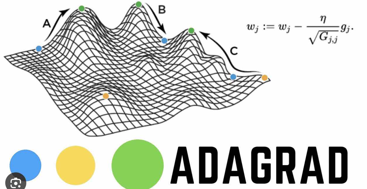
AdaGrad (Adaptive Gradient) is an optimization algorithm used in the field of machine learning and deep learning. It was proposed by John Duchi, Elad Hazan, and Yoram Singer in 2011. The algorithm adapts the learning rate for each weight in the model individually, based on the history of gradients.
Table of contents
Understanding Machine Learning and Optimization
Deep learning models operate within the paradigm of optimization, where we strive to minimize a cost function that represents the error of predictions on a given dataset. Optimization techniques like SGD, ADAGrad, RMSProp, and Adam are the backbone of deep learning, often making the difference between a mediocre and a highly accurate model.
Fundamentally, training a neural network involves finding the optimal set of parameters that minimizes a given cost function. While we aim to reduce the training error, the ultimate goal is to achieve a low test error — a measure of our model’s performance on unseen data. The cost function, often comprising a performance measure computed over the entire training set plus regularization terms, is vital for achieving this goal.
An integral aspect of the optimization process is the idea of learning indirectly. We use a different cost function to improve a performance measure defined with respect to the test set. Unlike pure optimization, where minimizing the cost function is the ultimate goal, deep learning optimization also pays attention to the structure of machine learning objective functions.
Many machine learning tasks can express the cost function as an average over the training set. For instance, the per-example loss function in supervised learning scenarios considers the predicted output given the input and compares it with the target output. This formulation defines an objective function concerning the training set. Optimally, we aim to minimize the equivalent objective function where the expectation is taken across the actual data-generating distribution, rather than just the finite training set.
We often encounter significant challenges when training deep learning models. The problem does not merely reside in optimizing the cost function, but also in the nature of the function itself. The task of training neural networks is not a convex optimization problem, making it significantly more complex.
One primary issue is the ill-conditioning of the Hessian matrix, a concept from convex optimization that reflects the curvature of the function. In the context of neural networks, ill-conditioning can cause the optimization process to stall, where even minuscule steps could increase the cost function. This issue arises when the curvature becomes so strong that it overpowers the gradient, slowing learning despite the presence of a strong gradient.
In this context, we will delve into an optimization method called ADAGrad. Unlike traditional algorithms like Gradient Descent, which utilize a single learning rate for all parameters, ADAGrad modifies the learning rate for each parameter based on the history of gradients. Adaptive learning rates are an essential feature of many modern optimization algorithms, offering a dynamic approach to parameter updates. This feature allows ADAGrad to handle data with sparse features more effectively, making it well-suited for Natural Language Processing (NLP) and Image Recognition tasks.
Also Read: Introduction to XGBoost and its Uses in Machine Learning
Stochastic Gradient Descent
Stochastic gradient descent is the simplest form of the optimization algorithm. Its strength lies in its simplicity and predictability: each step is directly proportional to the gradient at that point. It’s also susceptible to problems, like getting stuck in local minima and being sensitive to the choice of learning rate.
The update rule for SGD is given by:

Here, θ are the parameters we want to optimize, η is the learning rate, and ∇J(θ; x^{(i)}, y^{(i)}) is the gradient of the cost function J with respect to θ, computed for the i-th instance (x^{(i)}, y^{(i)}) in the training data.
This illustration shows the trajectory of the Stochastic Gradient Descent (SGD) algorithm in the optimization landscape. Each iteration represents a step towards minimizing the objective function, while the green dashed line illustrates the local gradient that guides the update.
From the above animation, we can observe that the point ‘bounces’ directly towards the minimum of the function, in a straight line. The algorithm is quite stable and finds the minimum, making it a good choice for simple problems or as a baseline. It lacks any form of acceleration or deceleration, which might be advantageous in more complex scenarios.
Also Read: What is Bayesian Optimization and How is it Used in Machine Learning?
Gradient Descent with Momentum
The gradient descent with momentum algorithm incorporates an element of ‘memory’ from previous gradients to accelerate the descent towards the minima. This method helps the algorithm navigate through ravines, where the surface curves much more steeply in one dimension than in another.
The update rule for Momentum SGD includes a velocity component v, which contributes to the final update direction.


Here, v_{t+1} is the current velocity, α is the momentum parameter, v_{t} is the velocity at the previous time step, and η \nabla J(θ_{t}) is the gradient of the cost function with respect to θ at time t.

This illustration represents the Momentum method’s optimization path. This momentum helps overcome shallow regions and local minima, making the learning process faster and more stable. The green dashed line represents the direction of the accumulated gradient.
From the animation, we can observe that the point doesn’t follow a straight line toward the minimum. Instead, it uses information from previous steps to build momentum in the steepest direction and dampen oscillations. This leads to faster convergence and less oscillation. Note: Larger steps in the parameter space can speed up the convergence of the optimization process, but they risk overshooting the minimum of the loss function.
ADAgrad
Adagrad is a more sophisticated optimization algorithm that adapts the learning rates for each parameter individually. This means that for each step of the training, each parameter can have a different learning rate. This can be particularly useful when dealing with sparse data, as Adagrad will assign a higher learning rate to infrequent parameters.
When exploring Variants of Gradient Descent, one must consider the distinctive role of Square Gradients in methods such as AdaGrad, where dealing with Infrequent Features becomes more feasible due to the adaptability of the learning rate in accordance with the Gradient Vector’s historical values.
Adagrad modulates the learning rates of all model parameters, scaling them inversely to the square root of the sum of all previously squared gradients (Duchi et al., 2011). This means that parameters associated with larger partial derivatives undergo a faster decrease in their learning rates, while those with smaller partial derivatives experience a slower decrease.

This is an illustration of AdaGrad optimization trajectory, which uniquely adapts the learning rate for each parameter based on the historical squared gradient values.
From the animation, you can see that Adagrad might converge slower compared to other methods. This could be because the accumulated gradient in the denominator causes the learning rate to shrink and become very small, thereby slowing down the learning over time.
Let’s take a look at the AdaGrad algorithm.
We start with AdaGrad, an algorithm that modifies the learning rate for every parameter θ_{i} at each step t based on the past gradients that have been computed for θ_{i}. It accomplishes this by applying an element-wise scaling of the gradient founded on the historical sum of squares in each dimension.
The algorithm initiates with an accumulation variable, r = 0, used to keep track of the sum of the squares of the gradient.
For each iteration, a minibatch of ‘m’ examples is sampled from the training set with corresponding targets.
The gradient, represented as ∇J(θ_{t}), is computed. Here, J is the cost function, and θ_{t} are the model parameters at the current iteration.
This gradient is squared and accumulated into r, following the update rule:

This helps us keep a running total of the sum of squared gradients.
Finally, the parameter update is applied using:

Here, η is the global learning rate and δ is a small constant introduced for numerical stability, typically around 10^-7. The square root and division are applied element-wise. This adjusts the model parameters, bringing us a step closer to the minimum cost function.
This process is repeated until the stopping criteria are met, incrementing ‘t’ for each new iteration. The algorithm’s aim is to adjust the parameters to find a local or global minimum of the cost function, reducing the discrepancy between the model’s predictions and the actual targets.
AdaGrad’s learning rate tends to become overly small when dealing with nonconvex functions or training neural networks, rendering it impractical for deep learning tasks. To rectify this, Hinton (2012) introduced the Root Mean Square Propagation (RMSProp) algorithm, a variant of AdaGrad that uses an exponentially decaying average to discard the extreme past. This adjustment allows the algorithm to converge more rapidly after finding a convex bowl as if it were an instance of AdaGrad initialized within that bowl.
Implementing the AdaGrad Optimization Algorithm from Scratch in Python
The script provided gives a comprehensive illustration of the AdaGrad optimizer in action. We first define the AdaGrad class, initializing it with a set learning rate and a small epsilon value for numerical stability. We then define an update method that implements the AdaGrad parameter updates, which is called during the training process.
The class works by initializing a gradient accumulator which stores the sum of the squared gradients for each parameter. When the update function is called, it first checks if the gradient accumulator is None (which it will be for the first call) and then initializes it with zero values the same shape as the parameters.
import numpy as np

class AdaGrad:
    def __init__(self, learning_rate=0.01, epsilon=1e-7):
        self.learning_rate = learning_rate
        self.epsilon = epsilon
        self.grad_accumulator = None

    def update(self, params, grads):
    """
    Updates the parameters according to the AdaGrad algorithm

    Parameters:
    params (dict): A dictionary containing parameters to be updated
    grads (dict): A dictionary containing gradients

    Returns:
    params (dict): Updated parameters
    """

        # Initialize gradient accumulator
        if self.grad_accumulator is None:
            self.grad_accumulator = {}
        for key, val in params.items():
            self.grad_accumulator[key] = np.zeros_like(val)

        # Update each parameter
        for key in params.keys():
            # Accumulate squared gradients
            self.grad_accumulator[key] += grads[key] ** 2
            # Update parameters with learning rate scaling
            params[key] -= self.learning_rate * grads[key] / (np.sqrt(self.grad_accumulator[key]) + self.epsilon)

    return params
In the main part of the script, we load and prepare the diabetes dataset from sklearn, standardize the features, add a bias column, and split the data into training and testing sets. We then define the model parameters, and functions to predict outputs, compute gradients, and compute loss.
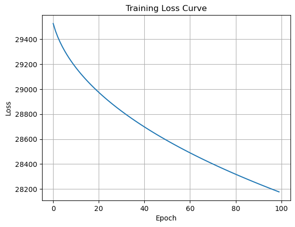
The AdaGrad optimizer is instantiated with a learning rate of 0.1, and the training process begins. In each epoch, we calculate the gradients using the compute_gradients function and then update the parameters with the update function from our AdaGrad optimizer. We compute and store the loss for each epoch. After the training, the training loss curve is plotted to visualize the decrease in loss over the epochs. This gives us a visual confirmation of the model’s learning process.
from sklearn.datasets import load_diabetes
from sklearn.preprocessing import StandardScaler
from sklearn.model_selection import train_test_split

# Load and prepare the dataset
diabetes = load_diabetes()
X, y = diabetes.data, diabetes.target

# Standardize the features
scaler = StandardScaler()
X = scaler.fit_transform(X)

# Add a bias column to the features
X = np.c_[np.ones(X.shape[0]), X]

# Split the dataset
X_train, X_test, y_train, y_test = train_test_split(X, y, test_size=0.2, random_state=42)

# Define the model parameters
params = {
"weights": np.random.normal(size=(X_train.shape[1],))
}

# Function to compute predictions
def predict(X, params):
    return X @ params["weights"]

# Function to compute gradients
def compute_gradients(X, y, params):
    predictions = predict(X, params)
    errors = predictions - y
    gradients = {
    "weights": 2.0 / X.shape[0] * X.T @ errors
    }
    return gradients

# Function to compute loss
def compute_loss(X, y, params):
    predictions = predict(X, params)
    errors = predictions - y
    return np.mean(errors**2)

# Instantiate the AdaGrad optimizer
optimizer = AdaGrad(learning_rate=0.1)

# Training loop
losses = []
for epoch in range(100):
    # Compute gradients
    grads = compute_gradients(X_train, y_train, params)
    # Update parameters
    params = optimizer.update(params, grads)
    # Compute and store loss
    loss = compute_loss(X_train, y_train, params)
    losses.append(loss)
    print(f"Epoch {epoch+1}, Loss: {loss}")

# Plot the loss curve
import matplotlib.pyplot as plt
plt.plot(losses)
plt.title("Training Loss Curve")
plt.xlabel("Epoch")
plt.ylabel("Loss")
plt.grid(True)
plt.show()
According to the epoch-wise loss outputs, our model’s performance improves consistently with each epoch. From Epoch 1 to Epoch 100, the loss value decreases from around 29525 to around 28177.
Epoch 1, Loss: 29525.430529088306
Epoch 2, Loss: 29466.23625907308
Epoch 3, Loss: 29418.291062806402
….
Epoch 99, Loss: 28184.085944841612
Epoch 100, Loss: 28177.07408407091
This code will give you a clear understanding of how AdaGrad impacts the model’s training process by showing the training loss curve.
Applications of ADAGrad
ADAGrad shines when it comes to dealing with sparse data. In machine learning and data science, sparse data refers to datasets where most features are zero for most samples. In NLP, the Bag of Words (BoW) or TF-IDF methods or even deep word embeddings can result in thousands or even millions of features, where each feature corresponds to a unique word in the vocabulary. In a given document, only a small subset of these words may appear, leading to a sparse feature vector. Similarly, in Image Recognition, especially with high-resolution images, each pixel can be a feature, leading to a high-dimensional and sparse feature vector.
This approach is advantageous as it allows for greater progress in more gently sloped directions of parameter space. Within the scope of convex optimization, AdaGrad offers several favorable theoretical properties. Training deep neural network models, it may result in a premature and substantial decrease in the effective learning rate due to the accumulation of squared gradients from the training’s onset. Therefore, AdaGrad performs well for some, but not all, deep learning models.
Challenges of ADAGrad
One of the primary limitations of AdaGrad is its aggressive decrease in the learning rate during training. AdaGrad adapts the learning rate for each parameter based on the accumulated sum of its gradients. As the sum of gradients can grow rapidly, the learning rate may diminish too much, too quickly, leading to premature convergence or extremely slow progress toward the end of training. This is especially a concern when training deep neural networks over numerous epochs.
AdaGrad’s performance depends heavily on the initial learning rate. If it is set too high, the learning rate may decrease rapidly early in the training, whereas a very low initial learning rate might result in a sluggish training process. Thus, AdaGrad requires careful tuning of the initial learning rate.
In spite of these challenges, AdaGrad’s concept of adapting the learning rate individually for each parameter is highly influential. It has inspired numerous adaptations and improvements, such as RMSProp and Adam, which have been found to perform better in deep learning tasks by overcoming some of AdaGrad’s limitations.
Also Read: How to Use Linear Regression in Machine Learning
Conclusion
In conclusion, the AdaGrad optimization algorithm presents a powerful approach to deep learning, effectively adapting the learning rates for all parameters based on their individual historical gradients. This unique feature can lead to improved performance, especially when dealing with data features that exhibit significant variability.
It’s crucial to remember that, like any algorithm, AdaGrad is not without its drawbacks. The notable issue of excessive reduction in learning rates and a pronounced dependency on the initial learning rate are challenges one might face when applying AdaGrad in real-world scenarios. Despite these, the fundamental idea of AdaGrad has catalyzed advancements in adaptive learning rate optimization methods, prompting the development of algorithms like RMSProp and Adam, which offer further enhancements.
Each of these optimization methods has its strengths and weaknesses, and it’s common to try out different methods and see which one works best for the problem you’re trying to solve. The choice of an optimization algorithm can significantly influence the efficiency and effectiveness of model training, so understanding the dynamics of these algorithms can be very valuable.

References
Bonaccorso, Giuseppe. Mastering Machine Learning Algorithms: Expert Techniques to Implement Popular Machine Learning Algorithms and Fine-Tune Your Models. Packt Publishing Ltd, 2018.
Santosh, KC, et al. Recent Trends in Image Processing and Pattern Recognition: 4th International Conference, RTIP2R 2021, Msida, Malta, December 8-10, 2021, Revised Selected Papers. Springer Nature, 2022.