Frequency Domain in AI

Introduction

The frequency domain in AI reframes signals as combinations of waves instead of raw time samples. This perspective reveals rhythm, periodicity, and hidden noise that ordinary time series views tend to obscure. Engineers use it to compress inputs, remove unwanted artifacts, and speed up heavy numerical computation. A Fourier based weather model named FourCastNet runs about 80,000 times faster than numerical prediction. Language research shows similar gains, with Fourier mixing reaching most of a transformer accuracy at lower cost. These results explain why spectral thinking now sits near the center of modern machine learning.

Quick Answers on the Frequency Domain in AI

What is the frequency domain in AI?

The frequency domain in AI describes data by the strength of its frequencies, letting models analyze spectra instead of raw time samples for faster, clearer pattern detection.

How is the frequency domain used in machine learning?

Models extract frequency features such as spectrograms, then feed them to networks for tasks like audio classification, forecasting, denoising, and fast physics simulation.

Why does the frequency domain speed up AI?

The fast Fourier transform mixes information in order n log n time, so spectral layers replace costly operations and cut training and inference cost.

Key Takeaways

• The frequency domain represents signals by frequency content, exposing periodicity and noise that plain time views often hide.
• Fourier transforms, wavelets, and the discrete cosine transform turn raw inputs into compact spectral features for models.
• Spectral methods such as Fourier neural operators deliver large speedups across weather, physics, audio, and vision tasks.
• Spectral bias and aliasing remain real limits, so frequency tools complement rather than replace time domain models.

What Is the Frequency Domain in AI?

The frequency domain in AI represents signals using their frequencies. It transforms raw time series data into spectral magnitude components. Models then read these spectra instead of raw temporal samples. This exposes periodicity, noise, and structure that clearly aids learning. Engineers apply this frequency domain view across many AI domains.

From Time Domain to Frequency Domain

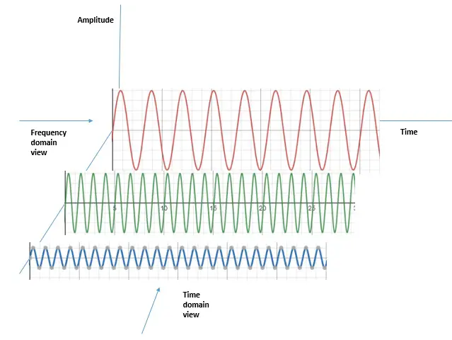
Every signal can be viewed in two complementary ways that describe the same underlying information. The time domain plots how a value changes from one moment to the next moment. The frequency domain instead measures how much of each repeating wave a signal contains. A pure musical note looks like a wavy line in time but a single spike in frequency. That spike marks the dominant pitch, while smaller spikes capture overtones and texture. Converting between the two views loses no information when the math is handled carefully.

Switching views often turns a messy time signal into a handful of clean, readable peaks. Speech, music, vibration, and sensor streams all carry periodic structure that frequencies expose well. A heartbeat trace, for example, hides a steady rhythm that a spectrum makes obvious. Sharp transient events spread across many frequencies, while slow trends concentrate near the low end. Reading these patterns helps networks described in basics of neural networks separate meaning from noise.

The conversion tool is usually the Fourier transform, an idea that dates back two centuries. It rewrites any signal as a weighted sum of sine and cosine waves. Digital systems use the discrete version, computed quickly by the fast Fourier transform. This algorithm made spectral analysis practical on ordinary computers and later on graphics hardware. Today the same math underpins audio codecs, medical scanners, and many modern deep learning layers. Each application relies on turning raw measurements into a clear map of frequencies. That shared foundation explains why one transform serves so many different fields.

Why Frequency Matters for Machine Learning

Frequency views give models a compact, structured signal that is often easier to learn from. Raw time series can be long, noisy, and full of redundant points that slow training. A spectrum compresses that stream into a few meaningful coefficients describing dominant rhythms. Models that compare machine learning versus deep learning often gain accuracy when fed spectral features. These features stay stable under small time shifts, which improves generalization across noisy samples. That stability matters when sensors drift or recordings start at slightly different moments.

Frequency framing also shortens the path between input and useful prediction in many tasks. A recent survey of frequency domain time series methods catalogs gains in forecasting, anomaly detection, and classification. Periodic demand, seasonal weather, and machine vibration all become simple peaks in a spectrum. Models then focus capacity on the frequencies that actually carry the predictive signal. The result is smaller networks that train faster and resist overfitting on limited data. Engineers can also inspect which frequencies a model weights most during prediction. This visibility turns an opaque model into a more transparent and trustworthy tool.

Putting Frequency Features Into Models

Building on that foundation, teams need a practical recipe for adding spectral features. The pipeline usually starts by slicing a long signal into short overlapping windows. Each window passes through a fast Fourier transform to produce a local spectrum. Stacking those spectra over time yields a spectrogram, a two dimensional image of frequency. That image becomes a clean input for convolutional networks or attention based encoders. The frequency domain in AI thrives on this image like representation of sound and motion.

Choosing the window length is the single most important tuning decision in this workflow. Short windows track fast changes but blur which exact frequencies are present. Long windows pinpoint frequencies precisely but smear the timing of quick events. This tradeoff, called the uncertainty principle, shapes every spectrogram a team produces. Engineers test several window sizes and overlaps before settling on a final configuration. Good defaults come from the sampling rate and the fastest event worth capturing.

Normalization follows, because raw spectral magnitudes span a very wide numeric range. Taking a logarithm compresses loud and quiet components into a comparable scale. Many teams also convert to a perceptual scale such as the mel spectrogram. These steps mirror the preprocessing used in spectral and rhythm audio classifiers. Careful scaling keeps gradients healthy and prevents a few bright bins from dominating training. Skipping this step often causes unstable loss curves and slow convergence. A short calibration pass on sample data usually reveals the best scaling choice.

Frequency features also support classic models when deep learning is overkill. A gradient boosted tree can read spectral energy bands as ordinary tabular columns. Forecasting tools shown in time series forecasting in Python accept these engineered features directly. This flexibility lets small teams adopt spectral methods without rebuilding their whole stack. The approach scales from a laptop notebook up to a production inference cluster.

Comparing Frequency Domain and Time Domain Approaches

Shifting focus to direct comparison, neither view is universally better than the other. Time domain models excel when exact ordering and sharp local events drive the outcome. Frequency domain models win when repeating structure and global patterns dominate the signal. Many strong systems combine both, reading raw samples and spectra in parallel branches. This hybrid design captures fast spikes and slow rhythms inside one shared network. Picking a starting point depends on the data, the latency budget, and the task.

The clearest split shows up in how each view handles noise and redundancy. Time models must learn to ignore noise spread thinly across thousands of samples. Frequency models can simply discard high bins where random noise tends to live. That pruning shrinks the input and often improves robustness on messy real recordings. Whether a network learns supervised or unsupervised, cleaner inputs help. The cost is a transform step and the risk of discarding useful detail.

Latency is another practical axis where the two approaches diverge sharply. A fast Fourier transform adds a small fixed cost before any model runs. For very short signals that overhead can outweigh the benefit of spectral features. For long sequences the transform pays for itself by collapsing redundancy fast. Teams should benchmark both paths on real hardware before committing to a design. The winning approach often mixes both views to balance accuracy against raw speed. Measuring that tradeoff early prevents painful and costly redesigns later in a project.

Fourier Transforms That Power Modern Models

Beyond feature engineering, the Fourier transform now lives inside the network itself. Researchers insert spectral layers that move data into frequencies, filter it, then return. These layers exploit the fast Fourier transform to mix information in order n log n time. A model named FNet replaces attention with a fixed Fourier transform. It reaches most of a strong transformer accuracy while training far more cheaply. The frequency domain in AI here becomes a computation trick, not just a feature source.

Spectral mixing works because a single transform connects every input position at once. Standard attention compares all pairs of tokens, which costs quadratic time and memory. A Fourier transform achieves global mixing without learning any pairwise weights at all. That parameter free design saves memory and speeds up very long sequence processing. The tradeoff is less flexibility, since the mixing pattern stays fixed across all inputs. Some hybrid models keep a little attention and add Fourier layers for cheap global reach.

Related work explores learnable spectral filters that adapt the fixed transform during training. Ideas like Fourier Analysis Networks let weights reshape frequency responses for each task. These designs aim to keep the speed of spectral mixing while regaining adaptability. Early results suggest competitive accuracy on language, vision, and scientific benchmarks. The field is moving quickly, with new spectral architectures appearing every few months. Many teams now treat spectral layers as a standard building block. Open libraries make these layers easy to drop into existing model code.

Fourier Neural Operators and Spectral Layers

Turning to scientific computing, spectral layers reach their fullest expression in neural operators. A Fourier neural operator learns mappings between whole function spaces. Each layer transforms the input, keeps the most important low frequencies, then transforms back. This lets one trained model solve a family of physics problems at many resolutions. The design is mesh independent, so a model trained on one grid runs on another. Such flexibility is rare among numerical methods and explains the surge of recent interest.

These operators shine on partial differential equations that govern fluids, heat, and waves. Traditional solvers march forward in tiny steps and consume enormous compute for fine grids. A spectral operator predicts the whole solution field in a single fast forward pass. The weather model FourCastNet uses adaptive Fourier operators for global forecasts. It approaches the accuracy of leading physics systems while running orders of magnitude faster. That speed opens the door to large ensembles that estimate forecast uncertainty cheaply.

The same machinery now supports faster weather and climate tools across research labs. Work on how AI improves weather forecasting shows spectral models spreading into operational settings. Energy planners use the rapid forecasts to schedule wind and solar generation more confidently. Disaster teams run many scenarios quickly to bound the path of a forming storm. Each use depends on the operator habit of capturing global structure through frequencies.

Spectral truncation, the act of keeping only low frequencies, is both strength and weakness. It removes noise and shrinks computation by ignoring tiny high frequency wiggles. Yet it can blur sharp fronts and fine textures that some predictions require. Researchers add correction terms or hybrid layers to recover the lost detail. The balance between speed and sharpness remains an active and lively research frontier. Practical systems blend truncated spectra with local corrections for the sharpest results. This pairing keeps the speed of operators while restoring crucial fine detail.

Frequency Domain Features in Audio and Vision

Among the clearest wins, audio and vision systems lean heavily on frequency domain features. Speech recognizers convert sound into mel spectrograms before any neural network sees it. Music tools described in AI generated music from wave data model audio directly through spectra. These representations expose pitch, timbre, and rhythm in a compact and learnable grid. Networks trained on spectrograms now power transcription, translation, and sound event detection. The frequency domain in AI made these audio breakthroughs both faster and more accurate.

Vision systems use frequency ideas more quietly, but the gains are just as real. Image codecs already store pictures as frequency coefficients through the discrete cosine transform. Feeding those coefficients straight into a network skips a costly decoding step. Models grounded in introduction to computer vision can read this compressed signal directly. High frequency components capture edges and texture, while low ones hold broad shape. Selective filtering of those bands can sharpen detection or defend against subtle attacks.

Risks and Limits of Frequency Domain AI

Despite the promise, spectral methods carry real risks that teams must respect. The best known is spectral bias, where networks learn low frequencies long before high ones. Research on the frequency principle in deep learning documents this consistent training pattern. Models therefore struggle to fit sharp edges, fine textures, and rapid oscillations. Tasks that depend on crisp high frequency detail can stall or look overly smooth. Engineers counter this with special encodings, multi scale training, or targeted loss terms.

Aliasing is a second hazard that silently corrupts spectra when sampling is too coarse. When a signal changes faster than the sampling rate, high frequencies masquerade as low ones. These phantom components mislead a model and are nearly impossible to remove afterward. Proper filtering before sampling, plus a high enough rate, prevents most aliasing. Window choice adds another artifact, since cutting a signal creates spurious frequency spread. Even basic functions like the softmax function cannot fix corrupted inputs.

Interpretability is a subtler limit that affects trust in spectral models. A spectrum is intuitive for engineers but opaque for many downstream stakeholders. Explaining why a frequency band drove a decision takes extra tooling and care. Spectral features can also leak sensitive patterns, such as identity cues in a voice. Teams must weigh these costs against the clear speed and accuracy benefits. Documenting these limits openly helps users trust the resulting predictions. Honest reporting also guides future work toward the hardest remaining problems.

Ethical Questions Around Spectral AI

Stepping back from pure engineering, spectral tools raise pointed ethical questions. Frequency analysis can reveal hidden traits in audio, video, and physiological signals. Voice spectra may expose age, health, or emotional state without explicit consent. Systems built on computer vision applications can read micro patterns people never intended to share. Responsible teams limit collection, anonymize spectra, and document every downstream use. Clear governance keeps powerful spectral analysis from drifting into quiet surveillance.

Synthetic media adds a sharper ethical edge to frequency based detection and generation. Generators often leave faint spectral fingerprints that betray artificial origin. Detectors that read those fingerprints, like methods in frequency domain learning research, help flag fakes. Yet the same knowledge teaches forgers how to hide their spectral traces. This arms race means detection tools need constant retraining to stay useful. Transparency about limits protects the public from false confidence in any single detector.

The Future of Frequency Domain AI

Looking ahead, frequency native models are likely to spread well beyond niche tasks. Foundation models for science already blend spectral operators with standard attention blocks. Researchers are exploring learnable transforms that adapt their frequency basis during training. Models explained in a weather prediction model explained simply hint at this direction. Such systems could forecast climate, traffic, and markets with far less compute. The frequency domain in AI is moving from a tactic toward a core design principle.

Hardware trends will accelerate this shift over the next several years. Modern accelerators compute fast Fourier transforms with dedicated and efficient units. As spectral layers become common, chips will optimize for them even more. Edge devices could then run spectral speech and sensing models on tiny power budgets. Cheaper transforms make real time spectral analysis feasible inside phones and wearables. That reach would bring frequency methods to billions of everyday devices.

Language and multimodal systems form another promising frontier for spectral ideas. Work near natural language processing suggests Fourier mixing can ease long context costs. Combining spectral mixing with sparse attention may unlock far longer inputs. Such models could read entire books or hours of audio in one pass. Expect rapid progress as these spectral and attention hybrids continue to mature. New research keeps lowering the cost of moving data into frequencies. That trend should push spectral methods into many more everyday products.

Key Insights

• FourCastNet generates a full week global forecast in under two seconds, roughly 80,000 times faster than numerical prediction (NVIDIA research).
• FNet reaches about 97 percent of strong transformer accuracy while training 70 to 80 percent faster using a fixed Fourier transform (Google Research).
• The frequency principle shows deep networks fit low frequency components first and high frequency detail last across training (Xu et al).
• Fourier neural operators learn mesh independent mappings between function spaces, so one model solves physics problems across many grid resolutions (neural operator overview).
• Audio classifiers convert clips into mel spectrograms and constant Q transforms before feeding these frequency images into convolutional networks (arXiv study).
• Learning in the frequency domain feeds discrete cosine coefficients into networks, cutting input data sharply while preserving classification accuracy (frequency learning paper).
• A 2025 survey catalogs frequency domain gains across forecasting, anomaly detection, and classification for modern time series models (time series survey).

These results point to one theme, that frequencies give models structure raw time often hides. Spectral features compress signals, expose periodicity, and speed computation across audio, vision, and science. Neural operators and Fourier mixing show the approach scaling from tiny sensors to global forecasts. The same physics that grants speed also brings spectral bias, aliasing, and interpretability costs. Treated as a complement to time models, frequency tools strengthen rather than replace them.

Dimension	Time Domain	Frequency Domain
Best for	Sharp local events and exact ordering	Periodic structure and global patterns
Noise handling	Must learn to ignore scattered noise	Can discard noisy high frequency bins
Input size	Long raw sample sequences	Compact spectral coefficients
Compute cost	Grows fast on long sequences	Order n log n with the fast transform
Periodic patterns	Hard to extract directly	Appear as clear single peaks
Sharp transients	Preserved precisely in time	Spread across many frequencies
Interpretability	Intuitive for ordered events	Clear to engineers, opaque to others
Typical models	Recurrent and causal networks	Spectral layers and Fourier operators

Frequency Domain Methods in Practice

In practice, several deployed systems show what spectral methods can actually deliver. Each example below pairs a concrete build with a measurable result and an honest limit. Real deployments prove that frequency thinking is far more than an academic curiosity. These cases span weather, language, and audio to show the breadth of impact. They also reveal the engineering effort that production spectral systems still demand. Read them as templates rather than guarantees, since every dataset behaves differently. Each project still demanded heavy tuning before it reached production quality. The payoff arrived only after teams matched the method to the right problem.

Global Weather Forecasting With FourCastNet

Researchers trained FourCastNet on decades of reanalysis data using adaptive Fourier operators. The team deployed it to produce global forecasts at a fine quarter degree resolution. Training finished in roughly sixty seven minutes on a large cluster, and inference saved enormous time. It generates a full week forecast in under two seconds, a dramatic increase in throughput. Accuracy still trails physics solvers for some sharp local variables that need fine detail. The documented results appear in the FourCastNet research paper for full review.

Faster Language Models With Fourier Mixing

Google researchers built FNet by replacing self attention with a fixed Fourier transform. They trained it on standard language benchmarks to test the parameter free mixing idea. The model reached about ninety seven percent of a strong transformer accuracy on those tasks. It trained seventy to eighty percent faster, a major increase in efficiency on long inputs. The fixed transform still limits flexibility, since it cannot adapt mixing per example. Full numbers and tradeoffs sit in the FNet paper from Google Research.

Audio Classification From Spectrogram Images

Engineers trained convolutional networks on spectrogram and mel feature images for sound tasks. They built pipelines that convert raw clips into time frequency pictures before classification. Reported accuracy rose by several percent compared with raw waveform baselines on the same data. The approach saved labeling effort because spectrograms made class boundaries visually clearer. Performance still required careful augmentation, since small datasets caused overfitting problems. The methods are detailed in a spectral audio classification study.

Lessons From Frequency Domain Deployments

Building on those wins, broader deployments reveal recurring lessons for new teams. Every successful spectral project paired strong math with disciplined data engineering. The case studies below avoid repeating the earlier examples and focus on distinct projects. They highlight medical signals, environmental sound, and efficient image pipelines in turn. Each one shows a measurable payoff alongside a limit that demanded extra work. Together they map the practical terrain that frequency adopters should expect to cross. Each team invested in data cleaning long before any model improved. That groundwork proved as important as the spectral math itself.

Case Study: Spectral Attention for Time Series

A research group built a complex valued spectral attention model for time series. They trained it to forecast and classify signals using bidirectional state space blocks. Reported error dropped by a clear percent margin against strong recurrent baselines. The spectral attention saved memory by mixing information directly in the frequency representation. Training still required careful tuning of the complex components to stay numerically stable. The full study appears in this spectral attention paper.

Case Study: Environmental Sound Recognition

A team deployed a deep classifier on urban and environmental sound recordings. They converted each clip into time frequency images and trained a lightweight network. Classification accuracy increased by several percent once spectral augmentation was added carefully. The pipeline saved compute because the small model ran well on modest edge hardware. Noisy field recordings still required hand cleaning before the model performed reliably. Details sit in an explainable audio analysis paper.

Case Study: Compressed Domain Image Learning

Engineers fed discrete cosine transform coefficients straight into convolutional vision networks. They built the pipeline to skip full image decoding before each training step. Input data shrank by a large percent while top line accuracy held steady. The shortcut saved bandwidth and sped up data loading across the training cluster. Models still required retraining, since standard backbones expect ordinary pixel inputs. The technique is documented in the learning in the frequency domain paper.

Common Questions About the Frequency Domain in AI