Recurrent Neural Networks (RNNs)

Introduction

Recurrent neural networks (RNNs) are the architecture that taught machines to read time itself, processing language, audio, and market data one step at a time. Before attention and transformers dominated headlines, these models powered the first wave of accurate speech recognition and machine translation. Google rebuilt its translation engine on recurrent layers in 2016 and cut translation errors by roughly 60 percent, according to the Long Short-Term Memory research record. That leap turned a research curiosity into infrastructure used by billions of people every day. This guide explains how the recurrent loop works, why it struggles with long sequences, and where it still wins in 2026. It compares LSTMs, GRUs, transformers, and state space models with current data and named case studies. By the end, you will understand both the mechanics and the strategic trade-offs that decide when to reach for a recurrent design.

Quick Answers on Recurrent Neural Networks

What is a recurrent neural network in simple terms?

A recurrent neural network is a model that processes data in order, using a hidden state to remember earlier inputs while reading later ones. This memory makes it ideal for text, speech, and time series.

What does RNN stand for and what is it used for in AI?

RNN stands for recurrent neural network. In AI it is used for speech recognition, language modeling, translation, handwriting recognition, and forecasting, anywhere the order of inputs carries meaning.

Are RNNs still relevant compared to transformers?

Yes, in niches. RNNs remain strong for streaming, low-latency, and edge tasks where inputs arrive one at a time and memory must stay small and constant.

Key Takeaways

• RNNs read sequences step by step and carry a hidden state that acts as memory of everything seen so far.
• Plain RNNs suffer from vanishing and exploding gradients, which LSTM and GRU gating mechanisms were designed to fix.
• Transformers overtook RNNs for large-scale language tasks, yet recurrent models still win on streaming and resource-limited workloads.
• State space models such as Mamba revive recurrent ideas with linear scaling and far faster inference than attention.

What Is a Recurrent Neural Network (RNN)?

Recurrent neural networks (RNNs) are deep learning models built for sequential data. They process inputs one step at a time across a sequence. A hidden state carries memory of earlier inputs forward. This recurrence captures order, context, and temporal dependencies well. They power speech, text, and forecasting tasks.

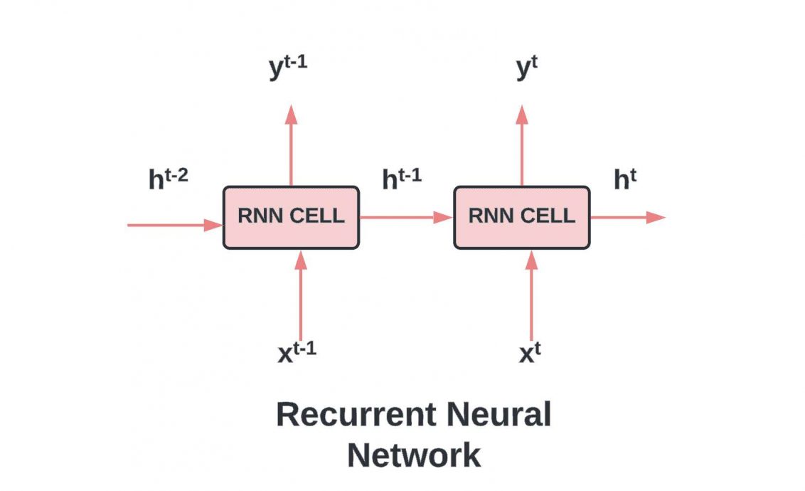
How the Recurrent Loop and Hidden State Work

A recurrent network processes a sequence by feeding each step's output back into the network as part of the next input. This loop is the defining feature that separates recurrent designs from every static model. At each time step, the network reads one element of the sequence, such as a word or a sensor reading. It then combines that element with a hidden state inherited from the previous step. The hidden state acts as a compact memory of everything the model has seen so far. By updating this memory at every step, the network builds context as the sequence unfolds. This simple mechanism lets the same set of weights handle inputs of almost any length.

The hidden state is a vector of numbers that the network rewrites on every step. Engineers initialize it to zeros, then let the data shape its values over time. One weight matrix transforms the previous hidden state, while another transforms the current input. The network adds these contributions and squashes the result through an activation such as tanh. A detailed Stanford recurrent network cheatsheet shows how this shared-weight structure drives efficiency. Because the weights repeat across steps, the model stays small even for very long inputs. That compactness made recurrent designs the default choice for sequence tasks for many years.

Information cycles through the loop until the sequence ends and the network emits its prediction. Some architectures produce an output at every step, which suits tagging and transcription work. Others read the whole sequence first, then generate a single label or a fresh sequence. This flexibility lets recurrent models handle translation, captioning, and forecasting within one framework. The basics of neural networks still apply, since each step is a familiar layer of weighted sums. What changes is the feedback connection that carries memory from one moment to the next. That feedback is both the source of the model's power and the root of its training trouble.

How RNNs Differ From Feedforward and Convolutional Networks

Feedforward networks treat every input as independent, while recurrent models treat inputs as an ordered stream. A standard feedforward network maps a fixed input to a fixed output with no memory between examples. That design works for tabular data or single images, where order does not matter. A recurrent network instead shares weights across time and threads a hidden state through the whole sequence. This lets it model dependencies that stretch across many steps, like grammar across a sentence. The difference is structural, not just a matter of tuning or scale.

Convolutional networks sit between these two extremes and capture local patterns through sliding filters. They excel at images and short signals where nearby values form meaningful shapes. Their receptive field stays limited unless engineers stack many layers to widen it. A recurrent network, by contrast, can in principle reference information from the very first step. Comparing these families clarifies why teams pick recurrent layers for ordered data and convolutions for spatial data. Understanding machine learning versus deep learning distinctions helps frame where each architecture belongs.

The Vanishing and Exploding Gradient Problem

Despite the elegance of the recurrent loop, training a plain RNN on long sequences is notoriously difficult. The trouble lives in how error signals travel backward through many time steps during learning. When the network unrolls across a long sequence, gradients multiply through dozens or hundreds of layers. If the repeated factors are smaller than one, the gradient shrinks toward zero and vanishes. If those factors exceed one, the gradient grows without bound and explodes into instability. Either failure stops the model from learning dependencies that span long gaps in the data.

Vanishing gradients are the more insidious of the two failure modes. They do not crash training, they quietly prevent the network from connecting distant events. A model might learn that nearby words relate while ignoring a subject mentioned ten words earlier. Exploding gradients are louder, producing wild loss spikes and numerical overflow during updates. Engineers tame the explosive case with gradient clipping, which caps the size of each update. The vanishing case demands deeper architectural fixes rather than a simple numerical patch.

Recent research argues the classic story is more nuanced than textbooks suggest. A 2024 analysis on vanishing and exploding gradients shows that growing memory makes outputs hypersensitive to parameter changes. As a network's effective memory increases, tiny weight shifts can swing predictions dramatically. This sensitivity makes gradient-based learning fragile even when gradients do not formally explode. The finding reframes long-sequence training as a stability problem, not only a magnitude problem. It also explains why careful initialization and normalization matter so much in practice.

These gradient pathologies shaped the entire history of recurrent modeling. They explain why plain RNNs rarely appear in production systems today. They motivated the gated cells that store information across long spans without decay. Techniques like batch normalization further stabilize deep recurrent stacks during training. Without these countermeasures, the promise of unlimited memory stayed mostly theoretical. With them, recurrent networks finally delivered on real language and speech tasks.

Long Short-Term Memory (LSTM) Networks Explained

Building on those gradient lessons, the LSTM cell became the most influential fix in recurrent modeling. Sepp Hochreiter and Jurgen Schmidhuber introduced it in 1997 to preserve information across long gaps. The cell adds a separate memory channel called the cell state that flows with minimal change. Three gates regulate that channel by deciding what to forget, store, and output. This gating lets gradients travel far back in time without vanishing into noise. The design turned long-range memory from a fragile hope into a dependable property.

Each gate is a small neural layer that outputs values between zero and one. The forget gate decides which parts of the old memory to discard at each step. The input gate chooses which new information deserves a place in the cell state. The output gate controls how much of the memory leaks into the visible hidden state. These learned valves let the network manage its own memory rather than overwrite it blindly. Activation choices like the sigmoid activation function make each gate smooth and trainable.

LSTMs dominated sequence modeling from roughly 2014 through 2018 across many domains. They powered machine translation, speech recognition, and handwriting systems at industrial scale. Their ability to hold context made them the backbone of early voice assistants. Even today LSTMs remain a strong baseline for modest datasets and streaming tasks. Their main cost is complexity, since each cell holds four times the parameters of a plain unit. That overhead motivated researchers to seek a lighter gated design with similar power.

Gated Recurrent Units (GRUs) and Why They Are Lighter

Turning to efficiency, the gated recurrent unit trims the LSTM down to two gates while keeping much of its strength. Kyunghyun Cho and colleagues proposed the GRU in 2014 as a streamlined alternative. It merges the cell state and hidden state into a single channel, which simplifies the math. An update gate decides how much of the past to keep against the new candidate state. A reset gate decides how much past context to ignore when forming that candidate. With fewer gates, the GRU trains faster and uses less memory than an equivalent LSTM.

In practice the two architectures perform comparably on most benchmarks. GRUs often edge ahead on smaller datasets where their lean parameter count resists overfitting. LSTMs sometimes win on tasks demanding very precise long-term memory control. A helpful overview of gated recurrent units details how the reset and update gates interact. Teams usually try both and let validation results pick the winner. This pragmatic bake-off remains good advice for any recurrent project in 2026.

Backpropagation Through Time: How RNNs Actually Learn

Moving on to training, recurrent networks learn through a variant of backpropagation called backpropagation through time. The method unrolls the network across every step of the input sequence first. It treats each time step as a layer in one very deep feedforward network. The algorithm then computes the loss and propagates error gradients backward through all those steps. Shared weights accumulate gradient contributions from every position where they were used. This accumulation is exactly where vanishing and exploding gradients arise during long runs.

Unrolling a long sequence is expensive in both memory and computation. Storing activations for thousands of steps can exhaust the memory of a single accelerator. Engineers use truncated backpropagation through time to cap the unroll length and control cost. This truncation processes the sequence in manageable chunks while carrying the hidden state forward. The trade-off is that very long dependencies beyond the window may be missed. Choosing the window length becomes a practical lever that balances accuracy against hardware limits.

Optimizers like Adam and RMSProp smooth the noisy gradients that recurrence produces. Careful weight initialization keeps early training stable before the model finds useful patterns. Loss design also matters, and studying PyTorch loss functions clarifies which objective fits a given task. Regularization such as dropout on recurrent connections curbs overfitting on small corpora. Together these techniques turn the fragile theory of recurrence into reliable training. Mastering them is the difference between a model that learns and one that stalls.

Sequence-to-Sequence Models and the Encoder-Decoder Design

Building on gated cells, the encoder-decoder design let recurrent networks map one sequence to another of different length. An encoder reads the full input and compresses it into a context vector that summarizes meaning. A decoder then reads that context and generates the output sequence one token at a time. This split made neural machine translation practical for the first time at large scale. The architecture also powers summarization, question answering, and speech-to-text transcription. It freed recurrent models from the rigid one-input, one-output mold of earlier designs.

The single context vector soon became the bottleneck of the whole approach. Squeezing a long paragraph into one fixed vector loses detail that the decoder needs. Researchers added an attention mechanism that let the decoder look back at every encoder step. This attention layer scored which input positions mattered for each output word. The fix dramatically improved translation quality on long and complex sentences. It also planted the seed that would later grow into the transformer architecture.

Attention turned the encoder-decoder from a memory test into a lookup system. The decoder no longer had to remember everything in one crowded vector. Instead it queried the encoder states directly whenever it needed specific context. This shift reduced the burden on the recurrent memory and lifted accuracy across benchmarks. Work on tokenization in NLP shaped how these models split text into trainable units. Good tokenization remains essential whether the backbone is recurrent or attention based.

Sequence-to-sequence systems proved that recurrent networks could generate language, not only classify it. They underpinned the first commercially successful translation and captioning products. Their structure still informs modern decoder designs even after attention took over. Understanding this lineage clarifies why transformers feel like a natural evolution rather than a clean break. Many ideas central to today's models were prototyped first inside recurrent encoder-decoder frameworks. That heritage is easy to forget amid the current excitement around attention.

Building and Training an RNN: Implementation in Practice

For teams ready to implement, building a recurrent model starts with shaping data into ordered sequences of fixed or variable length. Practitioners pad short sequences and batch them so the hardware can process many at once. They pick an LSTM or GRU layer, set the hidden size, and add a final dense layer for predictions. Frameworks such as TensorFlow and PyTorch provide these layers as a single line of code. A typical training loop feeds batches forward, computes loss, and applies backpropagation through time. Monitoring validation loss early helps catch overfitting before it wastes compute budget.

Tuning a recurrent model rewards patience and disciplined experimentation. Engineers sweep learning rates, hidden sizes, and dropout values to find a stable configuration. Gradient clipping guards against the explosive updates that plague long sequences. Whether deep learning is supervised or unsupervised shapes how labels and objectives are framed for the task. Reproducible seeds and version-controlled configs keep results trustworthy across runs. These habits separate a polished implementation from a fragile prototype that breaks under new data.

Where RNNs Are Used in Artificial Intelligence

Beyond the lab, recurrent neural networks (RNNs) sit inside products that millions of people touch every day. They transcribe voice commands, autocomplete text messages, and flag fraudulent transactions in real time. In healthcare, they model patient vital signs to predict deterioration before it becomes critical. In finance, they forecast demand, prices, and risk from streams of historical data. Each application shares one trait: the order of the inputs carries essential meaning. That ordering is exactly what recurrent designs were built to exploit.

Natural language processing was the first domain where these models reshaped the field. They powered language modeling, named-entity recognition, and sentiment analysis at scale. A clear primer on natural language processing shows how sequence models read meaning from word order. Anomaly detection systems use recurrent layers to learn the rhythm of normal behavior. When a new sequence breaks that rhythm, the model raises an alert. This pattern protects networks, factories, and payment systems from rare but costly events.

Autonomous systems also lean on recurrent memory to track motion over time. A self-driving stack may use recurrence to predict where pedestrians will move next. Robotics teams apply it to control loops that depend on recent sensor history. The common thread is streaming data that arrives one observation at a time. Recurrent models digest that stream without re-reading the entire past on every step. That constant-memory property keeps them attractive for embedded and real-time deployments.

RNNs for Time Series Forecasting and Prediction

Turning to numbers, recurrent neural networks (RNNs) became a workhorse for forecasting time series across industry. Analysts use them to predict stock prices, energy demand, and weather patterns from historical sequences. The gating in LSTMs lets the model weigh recent shocks against long-running seasonal trends. According to an Encord guide on time series predictions with recurrent networks, LSTMs handle temporal dependencies that simpler models miss. This strength made them a default baseline for financial and operational forecasting teams. Their predictions feed dashboards that guide real spending decisions.

Forecasting with recurrence still demands careful data work to succeed. Engineers must scale inputs, handle missing values, and avoid leaking future data into training. Comparing recurrent baselines against classical methods, like those in time series forecasting in Python, keeps expectations honest. Recurrent models can overfit noisy financial data and produce confident but wrong predictions. Robust backtesting on out-of-sample periods is the only reliable safeguard. Treating a forecast as a probability, not a certainty, prevents costly overreliance.

RNNs in Speech Recognition and Voice Assistants

Among the clearest wins, recurrent neural networks (RNNs) transformed speech recognition and the voice assistants built on it. Speech is a sequence of audio frames where context decides how each sound is interpreted. LSTMs learned to hold that context across long utterances and resolve ambiguous phonemes. This capability lifted transcription accuracy enough to make voice interfaces genuinely useful. The speech and voice recognition market reached USD 15.75 billion in 2025, according to SNS Insider market research. Recurrent models powered the foundation of that fast-growing industry.

Voice assistants combine several recurrent components into one responsive pipeline. A wake-word detector listens constantly for a trigger phrase using a tiny recurrent model. Once triggered, a larger network transcribes the request while tracking conversational context. Apple documented using recurrent architectures for its Siri voice trigger system. These models must run with low latency on phones with limited battery. That constraint is exactly where compact recurrent designs still outshine heavier alternatives.

Risks, Limitations, and Common Pitfalls of RNNs

Despite the strengths, recurrent neural networks (RNNs) carry real limitations that teams must weigh honestly. Their sequential nature blocks the parallel training that makes transformers so fast on modern hardware. Each step depends on the previous one, so the model cannot process a sequence all at once. This dependency makes training slow and expensive on very long inputs. Even gated cells struggle to retain detail across thousands of steps. For document-length context, attention-based models usually pull ahead in both speed and accuracy.

Overfitting is a constant risk, especially on small or noisy datasets. A recurrent model can memorize training quirks instead of learning general patterns. Without regularization, it may produce confident predictions that collapse on new data. Vanishing gradients still limit how far back a plain RNN can reliably look. These pitfalls explain why teams reach for LSTMs, GRUs, or attention rather than vanilla recurrence.

Deployment introduces a second class of practical problems. Recurrent inference is stateful, so serving systems must track hidden states across requests. A dropped or reordered packet can corrupt that state and degrade predictions silently. Debugging these failures is harder than inspecting a stateless model. Studying the natural language processing challenges teams face reveals many such operational traps. Planning for state management early prevents painful rewrites later.

Interpretability remains a stubborn weakness across recurrent systems. The hidden state mixes information in ways that resist clean explanation. When a forecast or transcription fails, tracing the cause is genuinely difficult. This opacity matters most in regulated fields like finance and medicine. Teams must pair recurrent models with monitoring, fallback rules, and human review. Treating the model as one component, not the whole system, contains the risk.

Ethical Considerations in RNN-Powered Systems

Stepping back from mechanics, recurrent neural networks (RNNs) raise ethical questions wherever they touch human lives. Speech recognition trained mostly on one accent can fail speakers of another. That gap can lock people out of voice-controlled services they depend on. Forecasting models can encode historical bias and then amplify it in automated decisions. When a credit or hiring system relies on biased sequences, harm scales quietly and fast. Engineers carry responsibility for auditing these effects before deployment, not after complaints arrive.

Privacy is a second pressing concern for sequence models. Speech and text data often contain sensitive personal details that demand protection. A model trained on private conversations can leak fragments of that data through its outputs. Strong governance, consent, and data minimization reduce this exposure substantially. Reviewing the broader historical overview of AI shows how repeatedly ethics lagged behind capability. Closing that gap is now a core part of responsible engineering.

Accountability rounds out the ethical picture for deployed systems. When an automated transcription mishears a medical instruction, someone must own the consequence. Clear documentation of training data, limitations, and intended use supports that accountability. Transparency reports help users understand when a recurrent model is making decisions about them. Independent audits catch failures that internal teams overlook under deadline pressure. Building these checks in early is cheaper than rebuilding trust after a public failure.

RNNs Versus Transformers and the Attention Revolution

Looking at the rivalry directly, transformers displaced recurrent neural networks (RNNs) for most large-scale language tasks after 2017. The transformer dropped recurrence entirely and processed every token in parallel through attention. This parallelism let models train on far larger datasets in far less wall-clock time. Attention also captured long-range dependencies that recurrence handled only with difficulty. The result was a step change in language quality that recurrent models could not match. Within a few years, the largest language systems were transformers almost without exception.

Transformers are not free, and their costs reopen the door for recurrence. Their attention operation scales quadratically with sequence length, which grows expensive fast. Doubling the input quadruples the compute and memory the model consumes. For very long streams or tiny edge devices, that cost becomes prohibitive. Recurrent models, with their constant per-step memory, remain attractive in exactly those settings. The choice is therefore about the workload, not about one architecture being universally superior.

The practical verdict in 2026 is a division of labor rather than a knockout. Transformers own large-scale text, code, and multimodal generation where parallel training pays off. Recurrent and recurrent-inspired models hold streaming, low-latency, and resource-limited niches. Research into geometric deep learning shows the field still values diverse inductive biases. No single architecture dominates every sequence problem worth solving. Smart teams match the tool to the constraint instead of following fashion.

The Future of Sequence Modeling: State Space Models and Mamba

Looking ahead, state space models revive the spirit of recurrent neural networks (RNNs) with modern mathematics and far better scaling. The Mamba architecture, introduced in the paper Mamba: Linear-Time Sequence Modeling, achieves linear scaling in sequence length. It delivers roughly five times higher inference throughput than comparable transformers. Crucially, its quality keeps improving on real data up to million-token sequences. This combination cracks the long-context problem that stalled both recurrence and attention. Mamba shows that selective, recurrent-style state can rival attention without its quadratic cost.

Hybrid designs now blend attention and state space layers to capture the best of both. A 2025 study in Scientific Reports combined transformer and Mamba components for stronger sequence modeling. These hybrids suggest the future is not recurrence versus attention but a thoughtful fusion. The recurrent idea of carrying compact state through time has clearly endured. What changes is the math that makes that state trainable and scalable. For long-sequence AI, the next decade may belong to these recurrent-inspired successors.

Key Insights on Recurrent Neural Networks

• Google rebuilt Google Translate on recurrent LSTM layers in 2016 and cut translation errors by roughly 60 percent, according to the LSTM research record.
• The global speech and voice recognition market reached USD 15.75 billion in 2025 and is projected to hit USD 143.20 billion by 2035 (SNS Insider).
• Automatic speech recognition software should grow from USD 6.82 billion in 2025 to USD 59.39 billion by 2035 at a 24 percent yearly rate (Market Research Future).
• The Mamba state space model delivers about five times higher inference throughput than transformers while scaling linearly with sequence length (Mamba paper).
• LSTMs introduced in 1997 added a gated cell state that lets gradients survive long sequences, taming the vanishing gradient problem (arXiv analysis).
• GRUs proposed in 2014 merged gates into update and reset controls, training faster than LSTMs with fewer parameters (GeeksforGeeks).
• A comprehensive 2024 review catalogs recurrent architectures and applications spanning language, speech, and time series forecasting (MDPI Information).

Taken together, these numbers show recurrent neural networks (RNNs) built the commercial foundation that later architectures now extend. They turned speech recognition and translation from research demos into multibillion-dollar markets within a decade. The same gating ideas that fixed vanishing gradients still inform today's state space models. Recurrence did not disappear when transformers arrived, it migrated into niches and inspired successors. The throughput gains of Mamba prove that compact, evolving state remains a powerful design principle. For practitioners, the lesson is to match the architecture to the data, the latency budget, and the sequence length.

Dimension	Plain RNN	LSTM	GRU	Transformer	Mamba (SSM)
Memory mechanism	Hidden state	Gated cell state	Merged gated state	Self-attention	Selective state
Long dependencies	Weak	Strong	Strong	Very strong	Very strong
Training parallelism	Sequential	Sequential	Sequential	Fully parallel	Parallel scan
Inference scaling	Linear	Linear	Linear	Quadratic	Linear
Parameter weight	Lowest	High	Medium	High	Medium
Best use case	Teaching	Streaming, modest data	Small datasets	Large-scale text	Long-context streams
Year introduced	1986	1997	2014	2017	2023
Long-context quality	Poor	Good	Good	Excellent but costly	Excellent and cheap

Recurrent Neural Networks in Action: Real-World Examples

Google Neural Machine Translation

Among the landmark examples, Google deployed an LSTM-based system called Google Neural Machine Translation in 2016. The team trained deep recurrent encoder-decoder layers on massive bilingual corpora. The system reduced translation errors by roughly 60 percent against the older phrase-based engine, as recorded in the LSTM history. That gain made machine translation usable for everyday communication worldwide. The model still struggled with rare words and very long sentences, which required later attention upgrades. This limitation showed that pure recurrence had a real ceiling on long-range fidelity. The example remains the clearest proof that recurrent networks could ship at planetary scale.

On-Device Voice Detection in Siri

In practice, Apple built recurrent models into Siri to detect its wake phrase and transcribe requests. Engineers trained compact LSTM networks that run directly on the device for privacy and speed. The approach kept wake-word latency low enough for natural conversation, as Apple described in its voice trigger research. On-device recurrence saved round trips to the cloud and protected raw user audio. The system still produced occasional false triggers and required tuning for diverse accents. That accent sensitivity highlighted a fairness limitation common to many speech models. The case shows why compact recurrent designs survive on battery-limited hardware.

Energy and Financial Demand Forecasting

Beyond consumer apps, analysts deployed LSTM models to forecast energy demand and financial time series. Trained on years of historical sequences, these models captured seasonality that simple linear methods missed. A DataCamp recurrent network tutorial walks through such a forecasting pipeline end to end. In production, well-tuned LSTMs cut forecasting error by double-digit percentages on some demand datasets. The models still overfit noisy financial data and required careful backtesting to stay reliable. That fragility limited their trustworthiness without strong validation guardrails. The example underscores both the promise and the discipline that forecasting demands.

RNN Case Studies With Measurable Outcomes

Case Study: Connected Handwriting Recognition

Researchers used deep LSTM networks to crack unconstrained connected handwriting recognition in the late 2000s. The models were trained on cursive samples where letters blur together without clear boundaries. These systems won several international competitions and reduced word error rates by double-digit percentages, as summarized in the LSTM literature. The breakthrough proved recurrence could segment and label messy real-world sequences. The approach still required large labeled datasets that were expensive to collect. That data hunger limited adoption for low-resource scripts and languages. The case established handwriting as an early recurrent success story.

Case Study: Early Clinical Deterioration Warning

Turning to medicine, hospitals piloted LSTM models that read continuous streams of patient vital signs. The networks were trained to flag deterioration such as sepsis before clinicians noticed it. In studies summarized in an MDPI review of recurrent applications, these models predicted risk hours earlier than standard scores. Earlier warnings gave care teams precious time to intervene and adjust treatment. The systems still generated false alarms that risked alert fatigue among busy staff. That noise required careful threshold tuning and human oversight to stay safe. The case shows recurrence saving time in high-stakes, streaming clinical data.

Case Study: Utility Energy Load Forecasting

Among infrastructure operators, utilities adopted recurrent models to forecast electricity load across daily and seasonal cycles. Engineers trained LSTM networks on years of metered consumption and matched weather data. Research in Applied Artificial Intelligence reports recurrent forecasters cutting error by meaningful percentages over classical baselines. Sharper forecasts let operators schedule generation and reduce costly reserve margins. The models still degraded during rare events like extreme weather absent from training. That brittleness required fallback rules and constant retraining to manage safely. The case highlights recurrence delivering measurable savings in operational planning.

Frequently Asked Questions About Recurrent Neural Networks