Univariate Linear Regression

Introduction

Univariate linear regression is one of the first algorithms anyone meets in machine learning, and it still does real work across data science today. The model draws a single straight line through data to predict one outcome from one input feature. Its simplicity hides genuine power, because the same math underpins forecasting, pricing, and risk scoring in production systems. Linear regression remains among the most widely used techniques in applied work, a point that GeeksforGeeks documents in its linear regression overview. Beginners reach for it because the link between input and output is easy to see and explain. Teams keep it because auditors and stakeholders trust models they can actually interpret. This guide walks through the formula, the training process, the evaluation metrics, and the ethical limits of the method. By the end you will know exactly where this simple model fits inside modern artificial intelligence.

Quick Answers on Univariate Linear Regression

What is univariate linear regression in simple terms?

Univariate linear regression predicts one continuous output from a single input feature by fitting a straight line, defined by an intercept and a slope, to the observed data.

What is the univariate linear regression formula?

The univariate regression formula is y = b0 + b1x, where b0 is the intercept, b1 the slope, x the single input feature, and y the prediction.

How is univariate regression used in AI?

It serves as a regression baseline and a building block for forecasting, trend estimation, and feature analysis inside larger machine learning and AI pipelines.

Key Takeaways

• Univariate linear regression models one output from one input using a straight line set by an intercept and a slope.
• Training finds the best line by minimizing mean squared error, using either gradient descent or the closed-form normal equation.
• Metrics such as R-squared and RMSE judge how well the fitted line explains and predicts the target variable.
• The method stays valuable in AI as an interpretable baseline, though its single feature and linear shape limit its reach.

What Is Univariate Linear Regression?

Univariate linear regression is a supervised learning method that models the straight-line relationship between one independent input and one continuous output, estimating an intercept and a slope so predictions minimize the squared error between predicted and actual values.

The Math Behind the Univariate Regression Formula

Building on that definition, the univariate linear regression formula gives the method its predictive shape and its name. The core equation is y = b0 + b1x, a straight line with two parameters that the algorithm learns from data. The intercept b0 marks where the line crosses the vertical axis when the input feature equals zero. The slope b1 measures how much the predicted output changes for each one-unit increase in the input. Because there is exactly one input feature and one output, the whole relationship lives on a flat two-dimensional plane. This is the structure people search for when they look up the phrase one input feature, two parameters, intercept and slope, one output. That single sentence captures the entire mechanical idea behind the model.

The two parameters are not guessed by hand; they are estimated so the line sits as close as possible to every training point. Each data point has an actual output value and a predicted value that the line produces for its input. The vertical gap between those two numbers is called the residual, or the prediction error. A good line makes these residuals small across the whole dataset, not just for a few lucky points. The model treats positive and negative errors symmetrically by squaring them before adding them up. Squaring keeps large mistakes from canceling small ones and punishes big misses more heavily. This idea connects directly to the cost function that the next section explains in detail.

It helps to ground the formula in a concrete picture before adding any heavier notation. Imagine plotting years of work experience on the horizontal axis and salary on the vertical axis for many employees. Univariate linear regression finds the one line that best summarizes how salary tends to rise with experience. The slope then reads as the average raise per extra year, and the intercept reads as the starting salary baseline. This same shape works for many tasks, which is why the model anchors so many introductions to supervised learning techniques and applied statistics. The formula is small, but its interpretation carries a lot of practical weight. Understanding it well makes every later concept easier to absorb.

How the Cost Function Measures a Poor Fit

Turning to the training problem, the model needs a single number that scores how badly a given line fits the data. That number comes from the cost function, and for univariate linear regression the standard choice is mean squared error. The cost function takes every residual, squares it, and averages the squared values across all training examples. Many textbooks divide this average by two as well, purely to make later calculus cleaner, as one walkthrough of the cost function and gradient descent explains. A perfect line that hits every point would score a cost of zero. A wildly wrong line produces a large cost because its squared errors pile up quickly.

Squaring the errors is the design choice that shapes the entire optimization process. It guarantees the cost is always positive, so the algorithm has a clear floor to move toward. It also makes the cost surface smooth and bowl shaped for a univariate model, which matters for the search method ahead. The single lowest point of that bowl corresponds to the best intercept and slope the data can support. Training is therefore a search for the bottom of this bowl rather than a guess about good values. Because the bowl has one minimum, the math is far gentler than the rugged loss surfaces seen in deep networks. That smoothness is exactly why this model is such a friendly teaching example for newcomers.

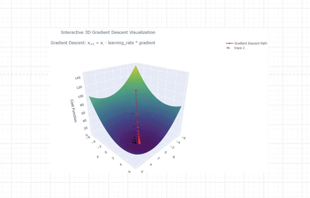
Gradient Descent and the Search for the Best-Fit Line

Beyond simply scoring a line, the algorithm needs a reliable way to improve it step by step. Gradient descent is the optimization method that does this, and it is the same engine that trains far larger models. The method starts with arbitrary values for the intercept and slope, often just zeros. It then measures the slope of the cost surface at that point, which is the gradient. The gradient points in the direction of steepest increase, so the algorithm moves the parameters in the opposite direction. Each small move lowers the cost a little, nudging the line toward a better fit. Repeating this loop many times walks the parameters down the bowl toward its minimum.

The size of each step is controlled by a setting called the learning rate, usually written as alpha. A learning rate that is too small makes training painfully slow, since each step barely changes anything. A rate that is too large can overshoot the minimum and bounce around without ever settling. Practitioners tune this value carefully, often testing several options before committing to one. A clear treatment from GeeksforGeeks on gradient descent in linear regression shows how the learning rate governs convergence speed. The bowl shape of the cost helps here, because there is only one minimum to find. That single minimum is what makes univariate regression so forgiving compared with deeper architectures.

Gradient descent updates both parameters at the same time on every pass through the data. The intercept and slope each have their own gradient, computed from the current errors across the dataset. The algorithm applies both updates together so the line shifts and tilts in one coordinated move. After enough iterations the changes shrink to almost nothing, signaling that the line has converged. At that point the cost is near its minimum and the parameters are considered trained. Engineers often plot the cost against iteration count to confirm a smooth downward curve. A jagged or rising curve is an early warning that the learning rate needs adjustment.

Gradient descent also scales gracefully when datasets grow too large to process at once. Variants such as stochastic and mini-batch gradient descent update parameters using small samples of the data. These variants trade a little stability for major gains in speed and memory use. The same logic later powers training for neural networks and many other models, as the basics of neural networks make clear. Learning the method here, on a simple line, builds intuition that transfers everywhere. That transfer of understanding is one reason this topic opens so many machine learning courses. Mastering it early pays dividends across the rest of the field.

Ordinary Least Squares and the Normal Equation

Shifting from iterative search to direct calculation, univariate linear regression also has a tidy closed-form solution. Ordinary least squares uses calculus to solve for the intercept and slope in a single step, with no looping required. It sets the derivatives of the cost to zero and rearranges the result into simple formulas. The slope equals the covariance of input and output divided by the variance of the input, while the intercept follows from the data means. This direct route is sometimes called the normal equation, and it gives exact parameters instantly. For a model with one feature and a modest dataset, this approach is fast, clean, and reliable.

The choice between the normal equation and gradient descent comes down to data size and structure. The closed-form solution shines for small problems where the math is cheap to compute directly. Gradient descent becomes the better tool once datasets grow huge or features multiply. The least squares method is also famously sensitive to extreme outliers that drag the line off course. A single rogue point with a large error can shift both the slope and the intercept noticeably. Knowing both routes lets practitioners pick the right one for each situation, a habit reinforced when getting started with machine learning in a structured way. Both paths, when applied carefully, land on the same best-fit line.

Univariate Linear Regression vs Multivariate and Multiple Regression

Stepping back from the mechanics, it helps to place this model among its close relatives. A univariate regression model uses exactly one input feature to predict one output, which keeps the picture two-dimensional. Multiple linear regression adds more input features, so a house price might depend on size, bedrooms, and location at once. Multivariate regression goes further by predicting several output variables together rather than just one. The naming trips up many learners, because the words sound almost interchangeable at first. A helpful clarification from Statology on univariate versus multivariate analysis hinges on the count of outcome variables. Counting inputs and outputs carefully resolves nearly every confusion here.

Each step up in complexity buys more flexibility at the cost of harder interpretation. A single-feature line is trivial to plot, explain, and defend to a non-technical audience. Adding features can improve accuracy when several factors truly drive the outcome together. That gain comes with risks like multicollinearity, where correlated inputs muddy the meaning of each coefficient. More features also raise the chance of overfitting, which careful validation work can help control. The simpler model is often the wiser starting point, even when richer data is available. Teams can always graduate to more features once the baseline is understood.

The family extends well past these three labels into many specialized cousins. Polynomial regression bends the line into a curve while still using linear coefficients underneath. Logistic and multinomial logistic regression adapt the framework to predict categories instead of continuous numbers. Tree-based methods such as decision trees drop the straight-line assumption entirely. Each variant solves a problem that pure univariate regression cannot handle on its own. Yet all of them echo the same core idea of fitting parameters to minimize error. That shared foundation is why the simple case deserves such careful study.

Interpreting the Intercept and Slope in Plain Language

Turning to interpretation, the real payoff of a univariate model is how readable its two numbers are. The slope tells you the expected change in the output for each one-unit rise in the input feature. A slope of 2,500 in a salary model means roughly 2,500 more dollars of pay per added year of experience. The intercept tells you the predicted output when the input feature sits at zero. Sometimes that zero point is meaningful, and sometimes it is only a mathematical anchor with no real-world reading. Stating units clearly keeps these interpretations honest and useful for decision makers.

Clear interpretation is exactly why regulated industries still favor this humble model. A loan officer can explain that each extra year of credit history lowers predicted risk by a stated amount. That kind of transparent reasoning is harder to extract from a deep network or from classification and regression trees. The slope and intercept turn a prediction into a sentence a human can challenge or trust. Analysts should always pair the numbers with a residual plot to confirm the line truly fits. Interpretation without diagnostic checks can mislead as easily as it informs. Treated with that care, the two parameters become a powerful communication tool.

Evaluating a Univariate Model with R-Squared and RMSE

Building on a fitted line, the next job is judging whether that line is actually any good. R-squared, also called the coefficient of determination, measures the share of variance in the output that the model explains. A value of 0.9 means the input feature accounts for ninety percent of the variation in the target. The metric ranges from zero to one for sensible models, with higher numbers signaling a tighter fit. A clear explainer from Arize on the coefficient of determination walks through how the score is computed. R-squared is intuitive, which is part of why analysts reach for it first.

R-squared alone can flatter a weak model, so it should never travel without companions. Root mean squared error reports the typical size of a prediction error in the original units of the output. A salary model with an RMSE of 4,000 dollars is easy to communicate to a business audience. Mean absolute error offers a similar reading while treating every miss in proportion to its size. RMSE punishes large errors more heavily because it squares them before averaging and taking the root. Reporting several metrics together gives a fuller, more honest picture of model quality. No single number can capture everything that matters about a fit.

Evaluation also depends heavily on how the data is split for testing. Scores measured on the same data used for training tend to look better than they truly are. Splitting data into training and test sets gives a more realistic estimate of future performance. For small datasets, repeated resampling through cross-validation to reduce overfitting stabilizes the estimate. Good evaluation habits matter as much for a simple line as for a giant network. Honest evaluation metrics are what keep even the simplest regression models genuinely trustworthy over time.

Core Assumptions That Keep the Model Honest

Turning to reliability, univariate regression rests on a handful of assumptions that quietly shape its trustworthiness. The first is linearity, meaning the true relationship between input and output really does follow a straight line. When the underlying pattern curves, a straight line will systematically miss in predictable ways. The second is independence, meaning each observation should not be tangled up with its neighbors. Time-ordered data often violates this, which is why forecasting needs extra care. Checking these assumptions before trusting the output separates careful analysis from blind curve fitting.

Homoscedasticity is the assumption most beginners overlook and most diagnostic plots reveal. It requires that the spread of residuals stays roughly constant across all levels of the input. When the spread fans out as predictions grow, the data shows heteroscedasticity instead. That funnel shape inflates the uncertainty around the estimated slope and intercept, as Statology on the four assumptions of linear regression details. A simple residual-versus-fitted plot exposes the problem at a glance. Analysts who skip this plot risk reporting confident numbers built on shaky ground. The fix often involves transforming the data or choosing a different model.

The third major assumption concerns the residuals themselves and their distribution. Classic inference expects the residuals to be approximately normally distributed around zero. You check the residuals, not the raw input or output, which surprises many newcomers. A histogram or a normal probability plot of residuals usually settles the question quickly. Mild departures from normality rarely break a model used purely for prediction. Serious skew, though, can distort confidence intervals and significance tests badly. Sound model building treats these checks as routine rather than optional.

Outliers deserve their own warning because least squares is so sensitive to them. A single extreme point can drag the entire line toward itself and distort both parameters. Standardized residuals greater than three in absolute value flag likely outliers for review. Removing or down-weighting such points must be done transparently, never silently to improve a score. Robust regression methods exist precisely to blunt the influence of these stubborn values. The lesson echoes the wider truth that clean inputs matter, a theme explored in how AI learns from datasets and data processing. Garbage in still produces garbage out, even for the simplest model.

Putting Univariate Regression to Work in Python

Moving on from theory, fitting a univariate regression in Python takes only a handful of steps. The scikit-learn library turns the whole modeling workflow into a few short, readable lines. You load your data with pandas and isolate one input feature and one target column. The library expects the input as a two-dimensional structure, so you reshape that single feature first. A simple train and test split then sets aside part of the data for honest evaluation. This compact recipe is why the model anchors so many first projects in linear regression in machine learning. Beginners can go from raw data to a fitted line within a single afternoon.

You create a regression object and call its fit routine on the training data. Behind the scenes the library solves for the intercept and slope using least squares. You then read the slope from the coefficient attribute and the intercept from its own attribute. Predicting on the test set gives values you compare against the truth using R-squared and RMSE. Clean inputs matter as much as clean code, a point reinforced by how data labeling for model performance shapes the final result. A tidy fit on messy data still produces misleading and fragile predictions in the end.

Validation is the step beginners skip and experienced practitioners never do. You plot the residuals against the predicted values to inspect the quality of the fit honestly. A shapeless cloud of points suggests the linearity and constant-variance assumptions both hold well. A clear curve or funnel shape warns that a single straight line is the wrong tool here. You also check for extreme points whose standardized residuals exceed three in absolute value. Only after all of these checks pass should the model inform any real decision.

Common Mistakes That Distort a Univariate Model

From there, a few avoidable mistakes quietly wreck more single-feature models than bad math ever does. The most common error is reading the intercept as meaningful when zero input never occurs in reality. A base salary at zero years of experience may be a pure artifact rather than a real figure. Analysts also forget to state units, which turns a clear slope into a genuinely confusing number. Mixing up the input and output axes flips the slope and reverses the entire interpretation. Skipping a quick scatter plot hides the curves that a single straight line can never capture.

Another frequent slip is trusting a high R-squared without ever checking the residuals first. A strong score can still hide a clear pattern that signals the wrong underlying model shape. Fitting and testing on the very same data inflates every metric and flatters a weak model. Sound practice always holds out a test set, a habit reinforced when getting started with machine learning the right way. Reporting many decimals of false precision also oversells what one lonely feature can truly deliver. Honest rounding keeps the model’s modest claims believable to a careful and skeptical reader.

Outliers cause the last common mistake, since one stray point can swing the whole line. Deleting awkward points silently to boost a score crosses from analysis into quiet dishonesty. The fair move is to document every excluded point and explain the reason for it plainly. Beginners also chase complexity far too soon instead of mastering the simple baseline first. A single-feature model, understood deeply, teaches lessons that transfer to every richer method later. Avoiding these traps matters far more than memorizing the underlying formulas by heart.

A final habit worth building is writing down the question before touching any data. A model fit without a clear goal tends to drift toward whatever pattern happens to look tidy. Stating the decision that the prediction will inform keeps the single feature honest and relevant. It also makes the eventual limitations far easier to spot and to communicate to others. Teams that skip this framing often ship a number that nobody can actually act upon. Clarity of purpose protects a simple model from quietly becoming a misleading one.

Where Univariate Regression Powers Real AI Systems

Beyond the textbook, univariate regression shows up far more often than its simplicity suggests. Teams use it as a baseline that any fancier model must beat before earning its complexity. Forecasting pipelines lean on single-feature trends to project demand, headcount, or energy use. Feature analysis often starts by regressing the target on one candidate variable at a time. These quick fits reveal which inputs carry real signal before a larger model is built. The method earns its keep as a fast, honest first pass through new data.

Interpretability makes the simple line a favorite for explaining model behavior to humans. Data teams use single-feature regressions to communicate a trend to executives in one chart. Monitoring systems track a slope over time to detect drift in a key business metric. Time-aware variants feed into broader pipelines, as shown in work on time series forecasting in Python. A clean linear relationship is often an early sign that the upstream data is healthy. That quiet diagnostic role is remarkably easy to underestimate in everyday production work. Engineers lean on it more than they usually admit in tutorials.

The model also anchors education and rapid prototyping across the whole field. Almost every course on common machine learning algorithms opens with this exact example. Prototypes use it to validate a pipeline end to end before swapping in heavier models. Its training cost is trivial, so experiments run in seconds rather than long hours. That speed lets teams test ideas about data plumbing without waiting on a deep network. The simple line becomes scaffolding that more ambitious systems are quietly built upon.

Risks and Limitations of Relying on a Single Feature

Turning to the downsides, leaning on one feature carries real and underappreciated dangers. A single input rarely captures the full story behind a complex outcome like price or health. Omitting an important variable can bias the slope and produce confidently wrong conclusions. Extrapolating beyond the range of the training data is another classic and costly trap. A line fit on incomes up to a point says little about incomes far outside that range. Treating a correlation as proof of cause is the most expensive mistake of all.

The model can also lull users into false confidence because its output looks so clean. A tidy equation invites trust even when the underlying relationship is not truly linear. Real-world phenomena often bend, saturate, or shift, defying any single straight line. When more factors clearly matter, a richer model or even deep learning approaches to AI may serve better. The honest move is to state plainly what one feature can and cannot explain. Pairing the model with diagnostics and domain knowledge keeps its limits clearly visible. Respecting those limits is what separates real analysis from wishful thinking.

Ethics, Fairness, and Responsible Use of Simple Regression Models

Stepping back from pure mechanics, even a simple line carries ethical weight when it touches people. A regression that sets insurance prices or screens applicants can encode unfair patterns from its data. If the single feature correlates with a protected attribute, the model can discriminate indirectly. Transparency helps, because a visible slope can be questioned in a way a black box cannot. Yet visibility alone does not guarantee fairness without deliberate testing across affected groups. Responsible teams test outcomes across those groups, not just the overall accuracy figure.

The interpretability of regression is an ethical asset only when teams actually use it. A clear slope lets an auditor ask why a feature drives a decision and demand a justification. That same clarity can expose proxies for race, gender, or income hiding inside an innocent variable. Documenting the data source, the assumptions, and the known limits builds real accountability. Stakeholders deserve to know when a prediction rests on one narrow and possibly biased feature. Cutting corners on this documentation undermines the very trust the model is meant to earn.

Fairness also depends on how predictions are used downstream by real decision makers. A model meant only for rough forecasting can cause harm if it is treated as a verdict. Human review should sit between a single-feature prediction and any high-stakes action taken. Teams should set thresholds for when a simple model is too thin to decide alone. The broader push for responsible systems threads through nearly every study of loss functions used in machine learning. Good governance treats even the simplest regression models as fully accountable decision tools.

The Future of Univariate Regression in Modern AI

Looking ahead, univariate regression is not going anywhere, even as deep learning dominates the headlines. Its role is shifting from headline solver to dependable baseline and trusted diagnostic tool. Automated machine learning platforms still fit simple regressions first to set a reference score. Explainable AI initiatives prize the model precisely because its internal logic is so transparent. As regulation tightens, interpretable models gain ground in finance, healthcare, and hiring decisions. The simple line is becoming a compliance asset rather than a dusty relic of the past.

The future of this model lies in pairing its clarity with the power of larger systems. Engineers increasingly use simple regressions to sanity-check the behavior of complex networks. A single-feature fit can flag when a deep model has latched onto a spurious trend. Hybrid workflows let teams enjoy both raw accuracy and human-readable explanation at once. The method also remains the gateway through which most people first meet the building blocks of neural networks. Its sheer teaching value alone almost guarantees the model a long life ahead.

Univariate linear regression will keep earning its place as the first model taught and the first baseline tried. Its math is gentle, its output is readable, and its assumptions are easy to check. Newer methods will keep winning accuracy contests on messy, high-dimensional datasets. Yet the need for models a human can explain only grows as AI spreads into daily life. A method that turns a prediction into a plain sentence will always have a job to do. That durable clarity is the quiet strength behind this enduring little algorithm.

Key Insights on Univariate Regression

• Arize explains the coefficient of determination as the share of variance explained, so an R-squared of 0.9 means one feature accounts for ninety percent of the output.
• The scikit-learn ordinary least squares example reports a mean squared error of 2548.07 and an R-squared near 0.47, proving how much a single feature leaves unexplained in practice.
• Statology lists the four assumptions of linear regression and notes that observations with standardized residuals above three in absolute value should be flagged as likely outliers.
• A widely cited cost-function and gradient-descent walkthrough divides mean squared error by two, a convention that makes the training derivative cleaner without changing the answer.
• GeeksforGeeks shows in its gradient descent guide that the learning rate alpha sets convergence speed, since a poor choice either stalls training or makes it diverge.
• Statology clarifies univariate versus multivariate analysis by the count of outcome variables, the single detail that resolves most of the naming confusion learners hit.
• Spot Intelligence recommends pairing RMSE with R-squared because root mean squared error reports typical error in the output’s own units, adding context a single ratio misses.

These insights point to one steady theme that runs through every section of this guide. A univariate model is powerful precisely because its single slope and intercept stay readable and auditable. The same simplicity that aids communication also caps how much variance one feature can ever explain. Sound evaluation, honest assumption checks, and outlier vigilance turn a fragile fit into a dependable tool. The model rewards discipline far more than it rewards raw computing power. Used with that care, it remains a trustworthy first answer in a crowded field of complex methods.

Univariate vs Multivariate Regression at a Glance

Given how often the naming confuses learners, a side-by-side comparison settles the differences fast. The table contrasts univariate, multiple, and multivariate regression across the dimensions that matter most in practice. Reading it row by row clarifies when each model earns its place. The comparison also highlights the trade-off between flexibility and interpretation that grows with every added variable. Keeping this map handy prevents the most common labeling mistakes. It also frames the modeling choices the rest of this guide explores.

Dimension	Univariate Linear Regression	Multiple Linear Regression	Multivariate Regression
Input features	Exactly one	Two or more	Two or more
Output variables	One	One	Two or more
Dimensionality	Two-dimensional line	Hyperplane in many dimensions	Multiple linked equations
Interpretability	Very high, easy to plot	Moderate, coefficients interact	Lower, harder to communicate
Overfitting risk	Low with enough data	Rises with feature count	Highest of the three
Computation cost	Trivial, closed-form available	Modest	Heaviest
Typical use	Baseline, teaching, quick trends	Realistic multi-factor prediction	Joint outcomes, such as multiple targets
Example	Salary from experience	House price from size, rooms, location	Predicting height and weight together

Univariate Regression in Action: Three Worked Examples

Predicting Disease Progression from One Clinical Feature

The scikit-learn project ran ordinary least squares on the diabetes dataset using a single body-mass-index feature to predict disease progression. The documented run trained the model on one input and produced a fitted line for the held-out test points. Its reported mean squared error lands at 2548.07, and the scikit-learn ordinary least squares example measures an R-squared near 0.47. That score means a single feature explains under half the variance in progression. The clear limitation is obvious here, because more than fifty percent of the signal stays unexplained by one variable. The example still earns its fame because it shows the workflow end to end in a few honest lines. It teaches both the power and the ceiling of a one-feature model at once.

Modeling Salary Growth from Years of Experience

A favorite teaching project builds a univariate model that predicts salary from years of experience alone. Practitioners trained the model with scikit-learn and read the slope as the average raise per added year of work. On the clean teaching dataset used in the DataCamp scikit-learn linear regression tutorial, the fit reaches an R-squared above 0.9, explaining over ninety percent of the salary variation. That high score reflects a tidy dataset built specifically to behave well. The limitation is that real salaries depend on role, location, and industry, so the neat line overstates its reliability. A model this clean rarely survives contact with messy production data. It remains a superb illustration of how readable a single coefficient can be.

Linking Advertising Spend to Sales

Marketing teams often deploy a single-feature regression to relate advertising spend to resulting sales. Analysts used the model to estimate how each extra dollar of spend tracks with revenue movement. As Arize illustrates with a sales example, an R-squared of 0.9 implies ninety percent of sales variation aligns with the modeled driver. That figure looks impressive and easily supports quick internal budget conversations with executives. The limitation is that advertising rarely acts alone, so seasonality and price changes can hide inside that score. Treating the correlation as proof that spend causes sales is the trap to avoid. The single feature is a starting hypothesis, not a final verdict on what drives revenue.

Case Studies in Applied Univariate Regression

Case Study: Retail Demand Planning from a Single Driver

Retail planners faced a recurring problem of stocking shelves without overcommitting cash to inventory. They needed a fast, explainable way to relate one strong driver, such as temperature or foot traffic, to daily demand. The teams built a univariate regression as a baseline before reaching for heavier forecasting tools, a pattern documented in a walkthrough of real-world linear regression examples. The fitted slope translated each unit of the driver into an expected change in units sold. In documented teaching cases the single-driver model can explain a large majority of short-run variation, often above 70 percent for weather-sensitive goods. The clear limitation is that promotions, holidays, and supply shocks fall outside one feature, so planners still overrode the model during unusual weeks. The baseline nonetheless cut guesswork and gave buyers a number they could defend. It remained a starting point rather than the final forecast.

Case Study: Lenders Screening Credit Risk with Regression Baselines

Lenders struggled with the problem of ranking applicants quickly while keeping decisions explainable to regulators. They needed a transparent first-pass screen before any complex scoring model entered the picture. Many introduced a simple regression linking one strong signal, such as credit history length, to a measured risk score. A 2025 study of R-squared in model accuracy places this application among common finance use cases, as a review of R-squared and model accuracy documents. The single coefficient let a loan officer state exactly how the signal moved predicted risk. Reported R-squared values in such baselines can reach roughly seventy percent of variance explained, supporting fast triage. The limitation drew real criticism, because one feature can act as a proxy for protected attributes and bake in bias. The baseline survived only as a screen feeding human judgment, never as the final lending decision.

Case Study: Forecasting Energy Use from Temperature

Utilities faced a persistent challenge of matching electricity supply to demand a day ahead. They needed a defensible model that planners and regulators could read without specialist training. Operators deployed a univariate regression tying outdoor temperature to load, a relationship that a guide to linear regression with real-world examples describes as a textbook single-driver fit. The slope captured how each degree of temperature shift raised or lowered expected consumption. On stable seasonal data the single feature explained a sizable share of daily variation, with reported fits commonly above 70 percent. The limitation appeared during heat waves and holidays, when the linear shape broke and errors widened sharply. Engineers still relied on the baseline for normal days while switching to richer models for extremes. The simple line earned trust as a daily workhorse, not a universal forecaster.

Frequently Asked Questions About Univariate Linear Regression