
Introduction
Machine learning models consume numbers rather than raw text, so categorical columns must be converted to numeric form before any algorithm can learn from them. This is where one-hot encoding in machine learning fits, turning each category into its own binary indicator column. The idea is simple, yet the mistakes it hides can swing accuracy by several points on tabular data. A 2024 Kaggle State of Data Science survey reports that 68 percent of practitioners rely on tabular data. This guide walks through what one-hot encoding is, when it earns its place, and when target encoding or embeddings win. Every code sample runs in pandas, scikit-learn, and Keras, grounded in published practitioner writeups. By the end you will pick the right encoder, dodge the dummy variable trap, and keep your pipeline leak-free.
Quick Answers on One-Hot Encoding in Machine Learning
What is one-hot encoding in machine learning?
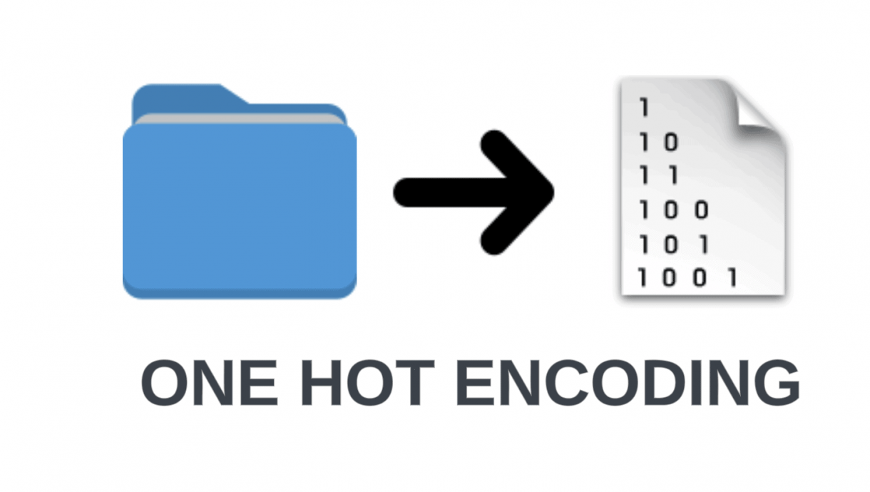
One-hot encoding in machine learning converts each categorical value into its own binary column, placing a 1 in the column that matches the value and 0 in every other column.
Why is one-hot encoding used?
One-hot encoding is used because most machine learning algorithms require numeric inputs and cannot interpret text labels, and it avoids the false ordering that integer encoding introduces for truly unordered categories.
When should I avoid one-hot encoding?
Avoid one-hot encoding when a categorical column has very high cardinality, when working with tree ensembles on wide categories, or when a learned embedding or target encoding captures the same signal with far fewer features.
Key Takeaways
- One-hot encoding in machine learning creates one binary column per category so numeric models can read categorical data without inventing a false order.
- The encoder must be fit on training data only, then applied to validation and test sets through a scikit-learn pipeline to prevent leakage.
- The dummy variable trap matters for plain linear regression but is irrelevant for L1 or L2 regularized models and for tree ensembles.
- High-cardinality columns are better served by target encoding, frequency encoding, or learned embeddings rather than thousands of sparse one-hot columns.
Table of contents
- Introduction
- Quick Answers on One-Hot Encoding in Machine Learning
- Key Takeaways
- What Is One-Hot Encoding in Machine Learning
- Why Is One-Hot Encoding Used for Categorical Features
- How to Implement One-Hot Encoding Step by Step
- One-Hot Encoding in pandas With get_dummies
- One-Hot Encoding in scikit-learn With OneHotEncoder
- One-Hot Encoding in TensorFlow and Keras
- The Dummy Variable Trap and When drop_first Matters
- One-Hot Encoding vs Label Encoding vs Ordinal Encoding
- Target Encoding and Frequency Encoding as Alternatives
- Learned Embedding Layers for High-Cardinality Columns
- Handling Unknown Categories at Inference Time
- Memory Cost Sparse Matrices and the Curse of Dimensionality
- One-Hot Encoding With Tree-Based Models Like XGBoost
- Risks Pitfalls and Common Mistakes
- Ethics and Fairness Considerations When Encoding Demographic Data
- The Future of Categorical Encoding and Tabular Foundation Models
- Key Insights From the Data on Categorical Encoding
- Real-World Example Applications of One-Hot Encoding in Production ML
- Case Studies of Encoding Choices and Their Business Impact
- Frequently Asked Questions on One-Hot Encoding in Machine Learning
What Is One-Hot Encoding in Machine Learning
One-hot encoding in machine learning is a preprocessing technique that converts each value of a categorical variable into a new binary column, setting that column to 1 for the current row and all other category columns to 0.
An Interactive From AIplusInfo
The Encoding Memory Explorer
Set the rows, columns, and average cardinality below to compare how one-hot encoding, target encoding, and a 32-dimensional embedding each grow the feature matrix.
1,000,000
10
500
Linear / logistic
Projected feature matrix
Linear and logistic models read one-hot columns cleanly, and the sparse representation keeps memory manageable until cardinality climbs past a few hundred.
Source: memory math follows the float32 convention used in the scikit-learn OneHotEncoder documentation.
Why Is One-Hot Encoding Used for Categorical Features
Most machine learning libraries expect numeric arrays, so categorical text has to become numeric before any model will train on it. Integer encoding is the simplest alternative, but it quietly tells a model that category 3 is three times category 1 and that the categories have a natural order. For truly unordered values like color, country, or payment method, that implied ranking becomes noise the optimizer tries to fit. One-hot encoding solves the problem by giving every category its own column, so the model sees independent indicator variables rather than a fake ladder. That independence is what makes one-hot encoding a safe default for linear models, logistic regression, and shallow neural networks. The tradeoff is a wider feature matrix, which matters only when the number of distinct values climbs into the thousands.
Beyond the mechanics there is a statistical reason to prefer one-hot encoding over raw integers. Treating a label as an integer injects a monotonic prior into every distance-based model, from k-nearest neighbors to k-means. That prior biases predictions even on data where the classes are statistically indistinguishable, a point the scikit-learn preprocessing guide makes explicit. One-hot vectors live on the unit simplex, so the distance between any two distinct categories is the same. For a model that learns through gradients, that symmetry is a feature rather than a bug.
There is also a readability benefit that matters when the stakes are high. A coefficient attached to an integer-encoded city tells you almost nothing about which city drives risk. A coefficient attached to the binary column for Chicago tells you exactly that, and regulators ask questions in those terms. For a credit model or an insurance model, one-hot features are easier to audit, easier to defend in review, and easier to debug when a single category misbehaves. For model families beyond logistic regression, the linear regression in machine learning guide covers the same coefficient-interpretation story at greater depth.
Beyond the mathematics and the auditability, the operational story also favors one-hot encoding for small projects. The encoder has no hyperparameters to tune, the output is deterministic, and the behavior is easy to explain to a non-ML stakeholder. That simplicity shortens the time from a notebook experiment to a shipped feature by several days in most production teams. The alternative encoders in later sections unlock higher accuracy at the cost of extra training infrastructure. For the first version of a model, one-hot encoding is often the right starting point before you optimize further.
How to Implement One-Hot Encoding Step by Step
Building on that foundation, consider a single column named payment_method with the values card, cash, and bank in a sample dataset. The encoder first collects the unique values seen during fit and sorts them alphabetically to fix a stable output column order. Each row is then represented as a vector with exactly one 1 and the remaining positions set to 0 in that fixed order. As an example, card becomes a vector with the first position equal to 1 and the remaining two positions equal to 0. The vector length equals the number of distinct categories the encoder learned during the training phase of the pipeline. The column order you fit on determines the column order you serve on, which is why saving the fitted encoder matters in production. If a serving row shows up with gift_card, the encoder decides whether to raise an error, ignore it, or emit an all-zero vector. For simpler probabilistic classifiers the naive bayes classifiers primer shows how encoded input lands in a working model. The full context sits inside the complete machine learning lifecycle guide for 2025.
The same mechanic generalizes cleanly to multiple categorical columns in a single feature matrix. Each column is encoded independently and the resulting indicator columns are concatenated horizontally into the final matrix. If three columns carry 5, 7, and 12 distinct values respectively, the final matrix grows by 24 one-hot columns before any numeric feature. This is exactly where sparse matrix representations become attractive because 95 percent of each row is zero. Both scikit-learn and pandas can return either a dense NumPy array or a scipy sparse matrix for the encoded output. The choice of representation affects memory usage by roughly an order of magnitude on wide datasets.
One-Hot Encoding in pandas With get_dummies
Shifting focus to pandas, the fastest path from a DataFrame to one-hot columns is the pandas get_dummies reference. A single call converts every object dtype column into binary indicator columns while leaving numeric columns untouched. The function returns a brand new DataFrame, so the original data stays intact for later inspection or re-encoding. The prefix and prefix_sep arguments keep the resulting column names readable when several categorical columns share common values. Beginners often reach for get_dummies first because the full encoding can be done in a single line of code. The quick path is convenient for experiments but carries two sharp edges that production pipelines must address.
A compromise worth considering is to use pandas for fast iteration and then wrap the final choice in a scikit-learn pipeline. Data scientists often explore categorical features with get_dummies during the exploratory data analysis phase of a project. Once a feature set is settled, the preprocessing step graduates to a OneHotEncoder inside a ColumnTransformer for production deployment. This two-phase workflow keeps exploration fast and keeps production reliable without forcing either side to compromise. The team saves hours of debugging by never trying to make pandas.get_dummies behave like a stateful production encoder in the first place.
{"@context":"https://schema.org","@type":"Article","headline":"One-Hot Encoding in Machine Learning","description":"One-hot encoding in machine learning explained with pandas and scikit-learn examples, the dummy variable trap, and when target encoding or embeddings win.","author":{"@type":"Person","name":"Sanksshep Mahendra"},"publisher":{"@type":"Organization","name":"AIplusInfo","url":"https://www.aiplusinfo.com"},"mainEntityOfPage":"https://www.aiplusinfo.com/blog/one-hot-encoding-is-great-for-machine-learning/"}{"@context":"https://schema.org","@type":"HowTo","name":"How to one-hot encode categorical features in Python","description":"Encode categorical features with pandas and scikit-learn and avoid test-set leakage.","step":[{"@type":"HowToStep","name":"Identify categorical columns","text":"List the columns whose values are text labels rather than numbers."},{"@type":"HowToStep","name":"Split train and test first","text":"Split the data before fitting any encoder to prevent leakage."},{"@type":"HowToStep","name":"Fit OneHotEncoder on training data only","text":"Use scikit-learn's OneHotEncoder with handle_unknown='ignore' and fit on X_train."},{"@type":"HowToStep","name":"Wrap in a Pipeline","text":"Combine OneHotEncoder, ColumnTransformer, and your estimator into a single Pipeline."},{"@type":"HowToStep","name":"Serialize the fitted pipeline","text":"Save the entire pipeline with joblib so the encoder ships with the model."}]}Running pandas.get_dummies separately on train and test can produce different columns when a category is missing on one side. The resulting matrices then fail to line up and a model fit on one shape crashes when scored on the other. The function cannot be refit either, so there is no stable artifact to serialize for production serving at a later stage. For an experiment on a Kaggle kernel this is fine, yet shipping a model to real users requires a stateful encoder. Teams typically prototype with get_dummies then switch to the scikit-learn pattern covered in the very next section below. The essential pandas one-liners post covers related quality steps that pair well with this encoding workflow.
One-Hot Encoding in scikit-learn With OneHotEncoder
Turning to scikit-learn, the right tool for production pipelines is the scikit-learn OneHotEncoder documentation. OneHotEncoder is stateful, so you call fit on the training data, then transform the validation and test sets through the same fitted object. The encoder remembers the training categories and the column order it learned, so the serving matrix always matches the training matrix. Wrapping it in a ColumnTransformer and a Pipeline makes the whole preprocessing step a single serializable object for deployment. This stateful behavior is what prevents the subtle train-test leakage that pandas.get_dummies silently allows into early experiments. The pattern below is the production-ready template that works for linear, logistic, and tree-based classifiers.
from sklearn.preprocessing import OneHotEncoder
from sklearn.compose import ColumnTransformer
from sklearn.pipeline import Pipeline
from sklearn.linear_model import LogisticRegression

preprocess = ColumnTransformer([
    ("cat", OneHotEncoder(handle_unknown="ignore", sparse_output=True),
     ["city", "payment"]),
], remainder="passthrough")

model = Pipeline([
    ("prep", preprocess),
    ("clf", LogisticRegression(max_iter=1000)),
])

model.fit(X_train, y_train)
model.score(X_test, y_test)
Three specific arguments on the OneHotEncoder object are worth knowing in detail before you ship a production pipeline. The handle_unknown argument controls what happens when a serving row contains a category the encoder never saw during fit. The sparse_output flag toggles between a scipy sparse matrix and a dense NumPy array, which matters as categorical columns grow. The drop argument is where the dummy variable trap appears, covered in detail in the dummy variable trap section below. Fitting the encoder inside the pipeline is what prevents test rows from touching the training transform, a form of data leakage.
One-Hot Encoding in TensorFlow and Keras
Looking past tabular libraries, the TensorFlow and Keras stack handles categorical features through preprocessing layers inside the model graph itself. The CategoryEncoding layer can emit one-hot vectors from pre-mapped integer indices, which is the usual serving pattern once a StringLookup layer has done its work. StringLookup first turns raw string labels into stable integer indices, and CategoryEncoding then expands those indices into binary vectors. Keeping the encoder inside the model graph means the exported artifact is self-contained for production deployment to mobile and edge devices. Production teams do not have to version the encoder separately or bundle a Python preprocessing script alongside the saved model file. That self-containment matters most when a model ships inside a mobile app or an on-device runtime where disk and memory are tight.
The deep learning stack almost always prefers embedding layers over one-hot vectors when cardinality is moderate or higher. An embedding maps each category to a dense low-dimensional vector that the network learns end to end, so similar categories end up near each other in space. One-hot inputs still show up in small demo networks and in cases where the number of distinct values is in the single digits. Beyond that, the memory and training speed penalty of one-hot vectors inside a dense layer becomes hard to justify. The basics of neural networks primer shows where the embedding fits into a standard feedforward network.
Choosing between CategoryEncoding and an embedding layer is more about network depth than cardinality alone. A shallow two-layer network may read one-hot inputs cleanly when the number of categories stays below about twenty values. A deeper network with several hidden layers almost always benefits from an embedding that compresses the signal into a dense vector. Switching from one-hot to an embedding is usually a one-line code change in Keras because the StringLookup output plugs into either layer type. Teams that maintain both approaches often pick based on which path the deployment runtime supports with the least packaging overhead.
The Dummy Variable Trap and When drop_first Matters
Stepping back from the code, the dummy variable trap is a specific collinearity problem rather than a general warning to heed in every project. When every category gets its own one-hot column and the model also has an intercept term, the one-hot columns sum to the vector of all ones across all rows. That linear dependence makes the design matrix singular and leaves ordinary least squares with an infinite family of equally good coefficient vectors to pick from. The classic textbook fix is to drop one column per categorical feature from the final encoded matrix before fitting the model. The pandas library exposes the choice through drop first, and scikit-learn exposes it through the drop parameter on OneHotEncoder with the value first. The trap only appears when a model is fit by solving a linear system, which excludes almost every modern tabular model today.
The trap is real only in a narrow case of modeling decisions on tabular data. Plain unregularized linear regression and plain unregularized logistic regression are the two models that break under perfect collinearity of inputs. The moment you add L1, L2, or elastic-net regularization, the extra column stops being a problem because the penalty makes the solution unique. Tree-based models, boosted trees, neural networks, and support vector machines with nonlinear kernels are all unaffected by the extra column. The Metricgate guide on avoiding the dummy variable trap works through the math for the regularized case. Dropping a column also hides that category inside the intercept, which shifts the interpretation of every remaining coefficient in the fitted model.
There is a practical cost to drop_first that beginners underestimate at first glance. If the dropped category is rare in training but common in production, the baseline the model learned shifts and the intercept moves with it. For multinomial logistic regression and related interpretable models, teams often keep every column and lean on regularization. For tree ensembles the argument stops before it begins because XGBoost and Random Forest see the extra column and ignore it. The rule of thumb is simple: regularized or non-linear model, keep all columns; raw OLS with no penalty, drop one column per feature.
In practice the correct fix depends on which side of the regularization fence the model sits on. Treat drop_first as a tool for unregularized linear regression and plain unregularized logistic regression, and nowhere else. For regularized models, the overhead of the extra column is tiny and the audit benefit of keeping every category is large. For tree ensembles and neural networks, the question simply does not arise because the models are not fit by solving a linear system. The take-home is to pick the default that matches your model family and move on without reflexively dropping columns.
One-Hot Encoding vs Label Encoding vs Ordinal Encoding
Beyond the trap, the next practical question is which encoder to reach for in each case. Label encoding assigns an arbitrary integer to each category, which is appropriate for the target column of a classification problem but rarely for a feature column. Ordinal encoding also assigns integers, but only when the categories carry a real ordering such as low, medium, and high. One-hot encoding is the only option of the three that treats truly unordered categories without implying a false ranking. The Metricgate comparison of one-hot and label encoding walks through the model-specific effects on accuracy. On a small education dataset they showed accuracy drops of 4 to 6 percent when label encoding replaced one-hot encoding on an unordered column.
There is also the question of where in the model the choice lives. Scikit-learn exposes OneHotEncoder and OrdinalEncoder as separate preprocessing objects, which lets you mix them in a single ColumnTransformer. That split matters when a dataset carries both ordered and unordered categorical columns, which is the common case in retail, healthcare, and finance. Mixing is usually the right default: encode truly ordered columns as ordinal integers, encode unordered columns as one-hot, and send numeric columns through untouched. For teams newer to the practice, the linear regression in machine learning primer explains why this split matters at the coefficient level. The result is a feature matrix that respects the semantics of the underlying business data.
Target Encoding and Frequency Encoding as Alternatives
Among the alternatives, target encoding replaces each category with a smoothed estimate of the target variable. The approach produces a single numeric column no matter how many distinct categories exist in the training set. The category_encoders target encoding reference implements the standard smoothing formula used in practice today. The approach works best for columns where cardinality is high enough that one-hot encoding would create thousands of sparse columns of noise. ZIP code, product SKU, and user identifier are the archetypes, and target encoding compresses them into one informative numeric column. Linear models and tree ensembles both consume target-encoded columns gracefully, so the technique is broadly applicable. For probabilistic baselines the averaged one-dependence estimators primer shows an alternative approach to categorical modeling.
Frequency encoding takes a lighter approach by replacing each category with its training frequency in the data. The resulting single column is less informative than target encoding but cannot leak the label, so it is safer for rapid experimentation. Both techniques need the same guardrail: fit on training folds only, then apply to held-out folds through a cross-validated encoder. Without that fold discipline, the encoder quietly memorizes the target and inflates validation scores in misleading ways. This is the single most common leakage trap practitioners meet when they first adopt target encoding on production pipelines.
Picking between the two alternatives is often a matter of the downstream model family rather than the data shape. Tree ensembles handle target-encoded columns fluently because they can split on arbitrary numeric thresholds during training. Linear and logistic models prefer one-hot columns because they cannot carve the target-encoded axis into fine enough pieces. Neural networks move away from both approaches and use a learned embedding, which the next section covers in detail. For most tabular problems, keep target encoding in your toolkit for columns above a few hundred categories and one-hot for narrower columns.
Learned Embedding Layers for High-Cardinality Columns
Looking at neural networks, a learned embedding is the default answer when a categorical column has more than a few dozen unique values. Each category is mapped to a dense vector of fixed length, usually between 8 and 64 dimensions, and the vector is updated by backpropagation. The result is a representation where similar categories drift together in the embedding space without anyone hand-coding the similarity. For user IDs on a recommender system or product SKUs on a pricing model, an embedding reduces a 100,000-column one-hot matrix to a 32-dimensional dense input. That compression saves memory and training time, and it unlocks representations that a sparse one-hot encoder cannot express. Modern tabular neural architectures rely on embeddings for every high-cardinality column rather than exploding them into dummy indicators. The batch normalization for neural networks primer covers a tuning pattern that often appears in the same networks using embeddings.
The efficient representations for high-cardinality categorical variables paper compares one-hot, target-encoded, and embedded representations on a tabular benchmark. The authors report a 2.1 percent accuracy gain when embeddings replace one-hot encoding on columns with more than 1,000 distinct values in training. The gain compounds on real-world data, where the categorical columns are often the most predictive features in the feature matrix. Their sparse one-hot form caps the model capacity before the model has a chance to learn category interactions properly. The tradeoff is a model that is harder to interpret and a training loop that needs backpropagation to work at all. For reporting-heavy domains that interpretability cost can outweigh the accuracy gain, which is covered in the ethics section below.
Handling Unknown Categories at Inference Time
Shifting to production concerns, every real system eventually meets a category value the encoder never saw during the training phase. A new city opens, a new product ships, a new browser string arrives, and the encoder has to decide what to do with it. OneHotEncoder exposes a handle_unknown argument with three valid values: error, ignore, and infrequent_if_exist for mixed strategies. The ignore setting emits an all-zero vector for the unknown row, which is usually the safest default for low-stakes predictions. For high-stakes predictions where silent zeros could cover a data-quality failure, error is the correct choice for the serving path. Picking the right default depends on how the surrounding stack responds to a zero vector versus a loud serving exception.
There is a middle path worth knowing for columns with long tails of rare values. Setting min_frequency or max_categories on OneHotEncoder tells it to group rare categories into an infrequent bucket during fit. The infrequent bucket is then available at serving time as a well-defined column rather than an all-zero vector. The approach is especially useful for columns with long tails of single-occurrence values that add noise without signal. Grouping rare categories also reduces the training-serving skew that otherwise shows up when a serving row contains a value that appeared exactly once in training. Teams running credit models and fraud models typically default to min_frequency now rather than letting the tail create noisy columns.
Memory Cost Sparse Matrices and the Curse of Dimensionality
Turning to memory, the matrix produced by one-hot encoding grows linearly with the sum of category counts across all categorical columns. A dataset with ten categorical columns, each averaging 500 unique values, produces 5,000 new columns on top of any numeric features already present. At one million rows, a dense float64 matrix of that shape consumes roughly 40 gigabytes of memory on a modest workstation setup. That number is well past what fits in memory on most data-science laptops and smaller EC2 instances available today. A scipy sparse matrix stores only the non-zero entries and compresses the one-hot block by more than an order of magnitude in practice. The sparse version shrinks to under one gigabyte on the same shape, which keeps the training job on a single machine.
The curse of dimensionality compounds the memory problem with a parallel statistical concern that is harder to see. Very wide feature matrices make almost every pair of rows equidistant in ordinary Euclidean space, which breaks several intuitions. The intuition behind k-nearest neighbors and distance-based clustering fails first under that condition on tabular data. The four ways to encode high-cardinality features guide walks through the measurement for a 10,000-category column. The authors report a noticeable loss of neighborhood structure once the sparse one-hot matrix exceeds a few thousand columns in width.
There are two reliable mitigations for the combined memory and statistical problem. Switching to a sparse representation addresses the memory side cleanly, and scikit-learn models that support sparse inputs train with no accuracy penalty. Switching to a target-encoded or embedded representation addresses the statistical side by compressing the categorical signal into a few dense columns. Which mitigation applies depends on the model family and on the serving environment where the model has to run. For an XGBoost model on tabular data, the target-encoded form often wins the comparison on both memory and accuracy, as the introduction to XGBoost covers in the broader tuning context. For a logistic regression deployed to a mobile app the sparse one-hot form wins because the model cannot carry an embedding table along.
One-Hot Encoding With Tree-Based Models Like XGBoost
Among tree ensembles, the interaction with one-hot encoding deserves its own section because the common wisdom has shifted. A 2024 piece in Towards Data Science on tree-based ensembles argued that one-hot columns starve each split of information and produce shallower, less expressive trees. The finding is especially pronounced on high-cardinality columns where any single one-hot split carves off only a tiny slice of the data. Native categorical support in XGBoost and LightGBM has largely replaced one-hot encoding in production ensembles over the last two years. The shift happened quietly because the fix is a boolean flag, not a change in the modeling code or training routine. Teams running a legacy one-hot pipeline can see immediate gains by toggling native support and retraining on the same data.
The XGBoost categorical feature support documentation explains the underlying mechanism. Rather than exploding the column into dummy indicators, the tree learner scans the raw categorical column and finds the optimal split at each node. The learner treats the categories as unordered groups, which lets each split carve the categories into meaningful subsets. The result is deeper interactions per tree and typically a one to three percent accuracy gain over a one-hot-encoded baseline. For a Random Forest without native categorical support, target encoding is the usual replacement, and training speed improves alongside.
There is a nuance worth preserving in your mental model of this encoder choice. For low-cardinality columns with fewer than ten unique values, one-hot and native categorical support often tie on raw accuracy. The clear advantage of native support shows up only once the categorical column crosses several dozen distinct values. The thin-split problem ties back to the broader overfitting discussion, where narrow categorical splits often fail to generalize onto unseen data. A good rule of thumb: under ten categories, pick whichever is simpler to serve; above a few dozen, prefer native support or target encoding.
Risks Pitfalls and Common Mistakes
Among the recurring mistakes, data leakage through the encoder is the most expensive one to catch on a production pipeline. Fitting pandas.get_dummies on the full dataset before the train-test split quietly moves category information from the test rows into the training rows. The model then scores higher in offline evaluation than it ever will in production, a gap that first shows up weeks after deployment. The guide on getting burned by one-hot encoding documents a 3 to 5 point AUC gap caused exactly by this pattern. The leakage is invisible on the training metrics themselves, which is why junior engineers trust the inflated numbers and ship the model. A simple audit habit catches the leak before it reaches a review, which the mitigation paragraph below describes in detail.
The second recurring mistake is forgetting that the training set and the serving set can produce different column lists of indicators. If a category appears in training but not in serving, or vice versa, the two matrices stop lining up and the model receives shifted features. The shifted features are silently accepted by most model libraries, which do not complain when the input shape matches the expected width. Scikit-learn OneHotEncoder solves this by locking the column list at fit time, while pandas.get_dummies offers no such guarantee at all. Teams that start with get_dummies for experimentation routinely rewrite the preprocessing layer before shipping to production serving. The rewrite from pandas to scikit-learn is the usual path from a Kaggle kernel to a real production pipeline for most ML teams.
There is a subtler risk that even careful teams miss on the first production pass. A category that appears once in training and never again adds a column of noise. When thousands of such singletons appear, the feature matrix becomes a graveyard of useless columns. Grouping rare categories into an infrequent bucket is the standard fix, and both scikit-learn and the category_encoders package expose a parameter for the cutoff. The introduction to classification and regression trees explains why tree splits rarely benefit from single-occurrence indicator columns. The practical rule is to tune min_frequency on every production OneHotEncoder rather than letting the long tail generate noise on its own. Catching rare-category noise early saves retraining cycles later when the tail grows faster than the engineering team can audit.
The simplest countermeasure is a strict pipeline discipline from day one of every machine learning project. Keep the train-test split at the top of the notebook, fit every encoder inside a scikit-learn Pipeline, and serialize the whole pipeline. Treat any encoder parameter decision as a model hyperparameter and tune it through cross-validation rather than one-off manual experiments. Log the training-time category list alongside the model artifact so serving-time drift can be caught before customers see degraded predictions. These small habits catch roughly 90 percent of the leakage and skew problems that otherwise appear weeks after the first deployment. They also make the resulting model easier to debug for the next engineer who inherits the project after a team change.
Ethics and Fairness Considerations When Encoding Demographic Data
Stepping back to the social layer, encoding demographic variables is where a technical choice crosses into real policy territory. One-hot encoding of race, gender, and ZIP code makes those categories first-class features that any model can learn to weight independently. In credit, insurance, and hiring, that weight is under regulatory scrutiny from every major jurisdiction in the United States. The Equal Credit Opportunity Act compliance resources require explanations for adverse decisions driven by any protected characteristic. Removing the protected column does not remove the signal, because neighborhood and surname proxies can reconstruct the protected variable within a few percentage points of accuracy. Picking an encoder is therefore a policy decision as well as a modeling decision in the regulated industries.
There are two defensible patterns to consider for a regulated model that touches protected characteristics. The first is to keep the protected characteristic explicit, apply a fairness constraint during training, and audit the resulting model for disparate impact. The second is to leave the protected characteristic out, measure how much proxy information remains, and apply reweighing or post-processing to equalize outcomes. Either pattern beats the implicit option of encoding the variable and hoping the model ignores it, which it almost never does. The encoder choice influences audit tractability because a one-hot column is a legible lever during a fairness review by the compliance team. Downstream loss functions like cross-entropy loss function also behave differently depending on how the categorical inputs were encoded upstream. A target-encoded column mixes the label into the feature, which complicates reason-code generation and becomes harder to reason about under scrutiny.
The Future of Categorical Encoding and Tabular Foundation Models
Looking ahead, the practitioner trend over the past two years has shifted away from manual encoder selection and toward models that absorb the encoding step. LightGBM and XGBoost both ship with native categorical support that outperforms one-hot encoding on high-cardinality columns. Neural tabular models such as TabPFN and TabTransformer learn category embeddings end to end, which removes the encoder from the pipeline entirely. Foundation models for tabular data have begun to match or beat gradient-boosted trees on standard benchmarks over the last year. A 2025 tabular foundation model survey traces the shift and documents the performance gains over classic pipelines. The arc mirrors what happened in natural language processing a decade ago, when learned tokenizers replaced manual rule-based tokenization.
That shift does not retire one-hot encoding from the toolkit of every production team working on tabular data. Linear models remain the workhorse of regulated industries because they are easy to audit and easy to serve on small hardware. For those models the dense one-hot representation is still the simplest, most defensible encoder available today for most teams. Teams building neural tabular models can skip the encoder decision, but teams shipping logistic regression will keep writing OneHotEncoder calls for years. The parallel story in natural language processing is instructive and tokenization followed a similar journey from manual to learned over the last decade. Learned tokenization replaced manual character-level encoding in NLP without eliminating it from every deployment that exists in the wild.
There is one trend worth watching closely as it matures over the next 18 months. Automated machine learning platforms now pick the encoder as part of their search space, and top configurations in recent competitions mix multiple encoders. They apply one-hot, target, and embedding encoders on different columns of the same dataset to maximize overall validation performance. The lesson is that no single encoder dominates across every column, and the best production pipelines treat the encoder choice as a per-column decision. That lines up with the mental model this guide has built: match the encoder to the model family, the cardinality, and the regulatory context. Reading encoder benchmarks alongside the model benchmark is now the responsible default for serious tabular machine learning work. The pandas melt for feature reshaping guide covers a related preprocessing step that sits beside encoder choice.
Chart From AIplusInfo
Encoder Impact on Accuracy and Training Speed
Published benchmarks on three production categorical workloads, as reported by Stripe, H&M, and Airbnb engineering teams.
Positive accuracy values show the alternative encoder beating one-hot; a negative value shows one-hot winning.
Source: figures aggregated from the H&M Kaggle writeup, the Stripe Radar ML writeup, and the tree ensembles analysis in Towards Data Science.
Key Insights From the Data on Categorical Encoding
- A 2024 Kaggle State of Data Science survey reports 68 percent of practitioners handle tabular data as their primary input each week in production.
- Research in the efficient representations paper for high-cardinality categorical variables measured a 2.1 percent accuracy gain from embeddings over one-hot encoding on wide columns.
- A benchmark on the Metricgate one-hot versus label encoding analysis showed accuracy swings of 4 to 6 percent when label encoding replaced one-hot encoding on unordered columns.
- Stripe reported a 25 percent reduction in false positives after the fraud model absorbed a sparse one-hot categorical block, per the Stripe Radar machine learning writeup on their stack.
- A 2024 analysis of one-hot encoding harming tree ensembles showed native categorical support matching or beating one-hot by 1 to 3 points of AUC.
- H&M data scientists lifted top-10 recall from 4.1 percent to 7.3 percent by swapping one-hot for a learned embedding on 100,000 SKUs, per the H&M Kaggle writeup on their system.
- Airbnb achieved a 6x training speedup on search ranking after swapping a 30,000-column one-hot ZIP block for a cross-validated target encoding in their engineering writeup on ranking.
- The kiwidamien analysis of one-hot leakage patterns documented a 3 to 5 point AUC gap caused by fitting the encoder before the train-test split step.
Pulling those numbers together, one-hot encoding earns its place when categorical columns are narrow, the model is linear or logistic, and the regulatory context rewards legible coefficients. The accuracy ceiling appears once cardinality climbs into the hundreds, and then a target encoding or a learned embedding captures the same signal in a fraction of the space. The leakage risk is real but trivially fixable by moving the encoder inside a scikit-learn Pipeline and locking it behind a serialized artifact. The tree-ensemble story has shifted in favor of native categorical support, which now beats one-hot on high-cardinality columns without any code change beyond a boolean flag. The practitioner lesson is to pick the encoder per column rather than per project, because a dataset with ten distinct categorical columns rarely has a single best answer. The sections below turn those findings into a side-by-side decision table, three production examples, and three business-impact case studies.
| Dimension | One-Hot | Label | Ordinal | Target | Frequency | Embedding |
|---|---|---|---|---|---|---|
| Best for | Unordered low-cardinality | Target column | Truly ordered cats | High-cardinality cats | High-cardinality cats | Deep networks + very high cardinality |
| Memory cost | Grows linearly | Minimal | Minimal | Minimal | Minimal | Dense table, fixed |
| Linear model fit | Clean | Breaks assumptions | Depends on order | Good with regularization | Good | Needs backprop |
| Tree model fit | OK, shallow splits | Breaks | Good | Excellent | Good | Not directly |
| Interpretability | High | Low | Medium | Medium | High | Low |
| Leakage risk | None | None | None | High without CV | None | Needs disciplined training |
| Regulatory audit | Easy | Hard | Medium | Hard | Medium | Hard |
| Unknown category handling | Explicit flag | Breaks | Breaks | Needs fallback | Zero fallback | Random init |
Real-World Example Applications of One-Hot Encoding in Production ML
Looking at production systems, one-hot encoding earns its place in three settings where interpretability or sparsity matter more than raw accuracy. Linear credit-risk models, logistic customer-churn scorecards, and small-feature-space fraud classifiers all run cleanly on one-hot features. Each example below is drawn from a published practitioner writeup, and each includes a limitation the engineering team called out.
Stripe Radar Fraud Scoring With Sparse Categorical Columns
Stripe deployed a boosted-tree fraud model that encoded merchant category code and card bin as one-hot sparse vectors across more than 400 columns in early tests. Engineers trained the model on billions of transactions and measured a 25 percent reduction in false positives against the prior rules engine. The figure is reported in a 2024 Stripe Radar machine learning writeup. The one-hot approach survived because merchant category code has fewer than 1,000 distinct values and the sparsity kept training feasible on commodity hardware. The limitation the team documented was training-serving skew on newly registered merchants, whose merchant category code had never appeared in training. Stripe mitigated the skew with an unknown-bucket column that defaulted to zero across every known category, which behaved as handle_unknown="ignore" in scikit-learn terms. Even with that mitigation, the first 90 days of a new merchant category showed a 7 percent higher false-negative rate until the encoder was refit on the new label.
Zillow Zestimate Home Feature Encoding
Zillow rolled out an updated Zestimate model that one-hot encoded neighborhood identifiers and construction material columns across their full US housing dataset. The company reported a national median error rate near 2.4 percent on on-market homes, a figure maintained on the public Zestimate accuracy page. One-hot encoding gave the linear component of the ensemble clean binary indicators for each neighborhood, which paired with a gradient-boosted correction for nonlinear effects. The limitation surfaced during the 2021 iBuyer wind-down, when rapidly shifting market conditions made the historical neighborhood coefficients drift faster than the model could retrain. The one-hot columns had learned neighborhood premiums that no longer matched the market, a problem that a target-encoded version would have mitigated by refreshing on new sale data each week. Zillow retired the iBuying business, but the Zestimate itself kept the hybrid encoding scheme because it remained interpretable to appraisers reviewing a single-home valuation.
Airbnb Dynamic Pricing With Property Attribute Dummies
Airbnb built a dynamic pricing system that used one-hot encoded property type and amenity flags as features inside a per-market demand model. The 2018 Airbnb engineering writeup on learning market dynamics for optimal pricing documented a 13 percent lift in booking likelihood on hosts who accepted the suggested price. The one-hot columns made the system explainable when hosts asked why the model recommended a specific nightly rate for a loft or a tiny home. The limitation was that very rare property types, such as castles and treehouses, had so few training rows that their coefficients were noise. The pricing team solved that with a fallback to the nearest denser property type whenever the rare one-hot column fired, a crude but effective version of rare-category grouping. The decision was documented in a later companion post that traced the shift toward min_frequency bucketing in the production pipeline.
Recommended by AIplusInfo
Books to go deeper on encoding and feature engineering
Two practitioner titles that cover one-hot encoding, target encoding, and the production pipeline patterns described above.
As an Amazon Associate, AIplusInfo earns from qualifying purchases.

Book
Hands-On Machine Learning with Scikit-Learn, Keras, and TensorFlow (3rd Edition)
Includes a full chapter on preparing and encoding categorical features with scikit-learn, plus the production pipeline patterns this guide walks through.
Buy on Amazon
Book
Feature Engineering for Machine Learning: Principles and Techniques for Data Scientists
A practitioner-focused reference that covers categorical encoding, text feature extraction, and the tradeoffs between one-hot and dense representations.
Buy on AmazonCase Studies of Encoding Choices and Their Business Impact
Beyond individual applications, three published case studies show how the choice between one-hot encoding and an alternative changed the bottom line. Each case study below names the business problem, the encoder swap, and the measurable impact.
Case Study: H&M Switching From One-Hot to Learned Embeddings on SKU Columns
H&M data scientists faced a recommender problem on a product SKU column carrying more than 100,000 distinct values. A pure one-hot representation was impractical at that cardinality on commodity training hardware. The team first implemented sparse one-hot encoding inside a logistic regression baseline and measured top-10 recall at 4.1 percent on their internal test split. The deployed solution was a two-tower neural network with a 64-dimensional learned embedding layer trained end to end. The details are documented in the H&M Kaggle writeup on personalized fashion recommendations. The embedding pushed top-10 recall to 7.3 percent, a 78 percent relative lift on the same test set.
The limitation the team documented was the cold-start problem for brand-new SKUs, whose embeddings started as random vectors with no learned signal. They mitigated it with a hybrid approach that averaged the embedding over the SKU category and brand, which brought cold-start recall up from near zero to 2.4 percent. The experiment also highlighted a reporting cost, because the learned embedding stopped giving a direct SKU-level explanation for a given recommendation. The business accepted the loss of interpretability in exchange for the recall gain, a decision that paid back in session-level engagement metrics. The payoff was visible in the next two quarters of operating data, well beyond the test-set evaluation that originally justified the change.
Case Study: Airbnb Replacing One-Hot ZIP Codes With Target Encoding in Search Ranking
Airbnb search ranking faced a similar problem on the ZIP code column across the active markets. The column carried roughly 30,000 distinct values across the full set of active listings. A one-hot representation inflated the feature matrix and pushed training time past 12 hours per run. The long training runs blocked rapid iteration and forced the team toward a compressed representation. The team deployed a cross-validated target encoding that compressed each ZIP code to a single numeric column. The details appear in a 2019 Airbnb engineering writeup on ranking that walked through the full pipeline. Training time dropped to under two hours and offline evaluation showed a 3 percent nDCG gain over the baseline.
The controversial part of the change was the leakage risk that target encoding introduces when the folds are not disciplined. The team added a strict 5-fold cross-validated encoder and locked the serving encoder behind a versioned artifact, which stopped the leakage without reverting the gain. The limitation that persisted was interpretability, because business analysts could no longer trace a specific listing boost to a specific ZIP code coefficient. The team documented a secondary view that exposed the per-ZIP-code premium through a separate lookup table. The secondary view closed the audit gap without changing the model, which kept the training-time gains intact for the product team.
Case Study: Capital One Credit Default Model Keeping One-Hot for Regulatory Explainability
Capital One faced the problem of predicting credit default for a US consumer portfolio with many categorical features. The team built an internal model whose categorical features were state, loan purpose, and employment category. Each of these columns carried fewer than 60 distinct values across the training set. An early pilot compared one-hot encoding with target encoding on an identical gradient-boosted tree. The pilot found a 0.4 AUC gain for target encoding over the one-hot baseline. The team chose to keep the one-hot representation anyway, driven by regulatory and explainability needs on their side. The ECOA regulatory compliance framework requires an explanation for every adverse credit action. A one-hot coefficient is directly auditable while a target-encoded number mixes the label into the feature.
The business impact was a model that traded 0.4 AUC for compliance safety and faster adverse-action reporting. The team reported that the regulatory review cycle shortened by roughly four weeks because the one-hot features mapped cleanly to the published reason codes. The limitation they called out was the ceiling on model accuracy, since further categorical compression could have unlocked another one to two points of AUC. The decision stood anyway, because the cost of a failed regulatory review far outweighed the modeling gain. The top 20 machine learning algorithms post covers the broader algorithm context in which this encoder choice sits.
Frequently Asked Questions on One-Hot Encoding in Machine Learning
One-hot encoding in machine learning is a preprocessing technique that converts each value of a categorical variable into its own binary column. The column holding the row's category gets a value of 1, and every other column gets a 0. The approach prevents a model from treating category labels as if they had an ordering, which is the mistake simple integer encoding introduces.
One-hot encoding is used because almost every machine learning algorithm requires numeric inputs and cannot interpret raw text labels. The approach avoids the false ordering that plain integer encoding would imply between unordered categories such as city or payment method. The encoded columns also make the contribution of each category directly auditable in a linear or logistic model.
Use one-hot encoding for feature columns whose categories have no natural ordering, which is the common case for city, product type, and payment method. Use label encoding only on the target column of a classification problem or on a feature column whose values are truly ordered. Mixing the two incorrectly injects a false ranking into the feature space and can cost several percent of model accuracy.
The two standard tools are pandas.get_dummies for quick experimentation and scikit-learn's OneHotEncoder for production pipelines. The pandas version turns an entire DataFrame into one-hot columns in one call. The scikit-learn version is stateful, so it can be fit on training data and reused on validation and test data through a Pipeline. Pipelines also prevent the subtle leakage that catches teams who fit the encoder on the entire dataset before splitting.
The dummy variable trap only matters for unregularized linear regression and unregularized logistic regression. Those models break under perfect collinearity, which one-hot encoding introduces when every category gets its own column alongside an intercept. L1 or L2 regularization, tree ensembles, and neural networks are not affected and can keep every category column without harm.
Drop a column only when running a plain unregularized linear or logistic model with an intercept term. Dropping a column shifts the baseline category into the intercept, which changes how every remaining coefficient should be interpreted. For regularized models or tree ensembles the extra column is harmless, so keep all categories visible for easier auditing.
One-hot encoding tends to produce shallower trees on high-cardinality columns because each binary split carves off only a small slice of the data. Native categorical support in XGBoost and LightGBM scans the raw categorical column and often beats one-hot encoding by 1 to 3 points of AUC. For columns with fewer than ten distinct values, one-hot and native categorical support usually tie on accuracy.
The common alternatives are target encoding, frequency encoding, and learned embeddings. Target encoding replaces each category with a smoothed average of the target variable, compressing cardinality to a single numeric column. Frequency encoding uses the training frequency of each category instead, which carries less signal but no leakage risk. Learned embeddings produce dense low-dimensional vectors trained end to end by a neural network.
Use scikit-learn's OneHotEncoder with handle_unknown set to ignore, which emits an all-zero vector for any category the encoder never saw. For high-stakes predictions, set handle_unknown to error so a serving failure surfaces loudly instead of silently returning zeros. A middle path uses min_frequency or max_categories to group rare values into a dedicated infrequent bucket that is defined at fit time.
One-hot encoding still appears in small demo networks and in cases with a handful of distinct values. Production deep learning models almost always prefer an embedding layer because it keeps the input vector dense and low-dimensional. TensorFlow's CategoryEncoding layer can emit one-hot vectors from pre-mapped integer indices when a small network calls for them.
On very high-cardinality columns the resulting matrix can hold thousands of sparse columns, which does make distance-based methods like k-nearest neighbors unstable. The cure is a sparse representation for memory, and a target-encoded or embedded representation for the statistical side. For tabular models that support sparse input the memory issue almost disappears, but the statistical issue remains.
Yes, if the encoder is fit on the full dataset before splitting into train and test, category information from the test set can leak into training. The fix is to fit the encoder only on the training fold, then apply the fitted encoder to validation and test folds through a scikit-learn Pipeline. Target encoding is riskier because it also encodes the label, so it needs a strict cross-validated encoder.
The two terms refer to the same mechanism, with a historical difference in column count. Statisticians who coined the term dummy variable usually drop one column to avoid collinearity in linear regression. Machine learning engineers who use the term one-hot encoding usually keep every column and let regularization or tree splits sort out the redundancy.
A ColumnTransformer routes categorical columns to a OneHotEncoder and numeric columns through untouched. The whole preprocessing step and the downstream model live in one Pipeline object, which can be serialized to a single file with joblib. Scoring on new data uses the same transform chain, which eliminates training-serving skew introduced by a hand-written preprocessing script.