
Introduction
Classification and regression trees are still central to modern machine learning pipelines across industry today. Data scientists shorten the name to CART, and the algorithm still powers a large share of production models. Kaggle’s State of Data Science report, based on a survey of 23,997 practitioners in 2022, found that tree-based methods were the most widely used algorithms across working data teams. That popularity did not fade when transformers arrived, because CART remains easy to interpret and defend in regulated settings. This guide explains how CART works, how CART chooses splits, and how to tune, and prune trees in scikit learn without letting them memorize. You will see worked examples, three production case studies, an interactive tuner, and a chart of accuracy against tree depth. By the end you will know when to reach for a single tree and when to step up to random forest, XGBoost, or a neural network.
Quick Answers on Classification and Regression Trees
What are classification and regression trees in machine learning?
Classification and regression trees, or CART, are supervised models that split data into recursive binary regions and predict a class label for classification tasks or a numeric value for regression tasks.
How does a regression tree in machine learning differ from a classification tree?
A classification tree returns a discrete label and picks splits with Gini impurity or entropy. A regression tree returns a continuous number and picks splits by variance or residual sum of squares reduction.
When should you use classification and regression trees over other algorithms?
Use classification and regression trees when interpretability, non linear feature interactions, and mixed data types matter more than raw accuracy on a moderate sample size.
Key Takeaways on CART in Machine Learning
- CART is a supervised algorithm that builds a binary tree using recursive splits, and each split is chosen to reduce impurity or variance the most.
- Classification trees rely on Gini impurity or entropy, while regression trees rely on residual sum of squares, so the objective changes with the task.
- Single trees overfit quickly, and cost complexity pruning with ccp_alpha is the standard remedy in scikit learn for classification and regression trees.
- Random forest, XGBoost, and LightGBM all use CART trees as base learners, so the theory in this guide carries directly into modern ensembles.
Table of contents
- Introduction
- Quick Answers on Classification and Regression Trees
- Key Takeaways on CART in Machine Learning
- What Is a Classification and Regression Tree in Machine Learning
- How CART Fits Into the Wider Machine Learning Landscape
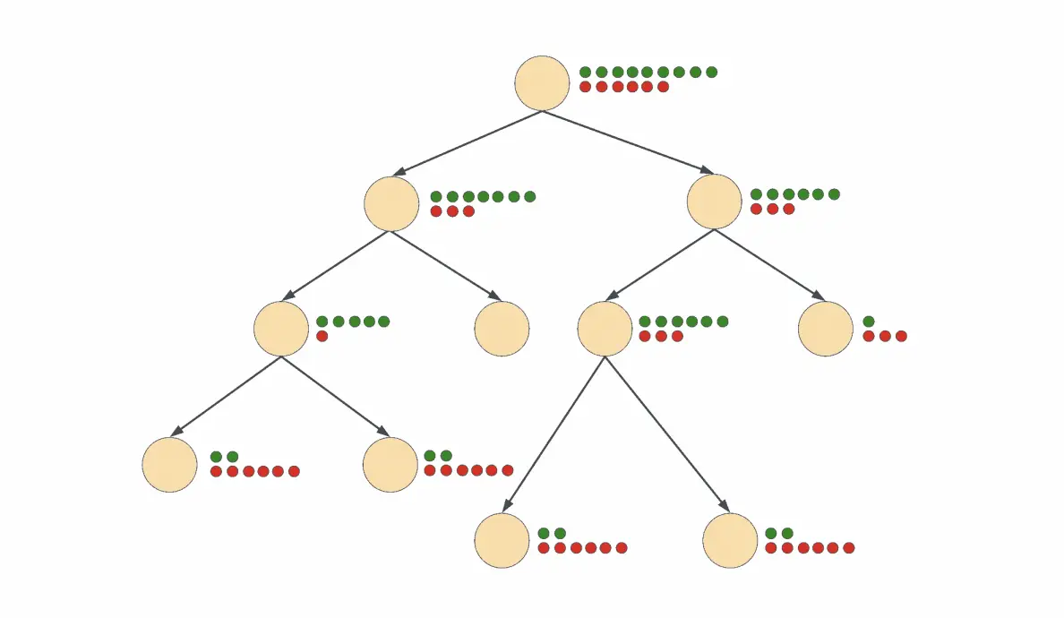
- The Anatomy of a Decision Tree Built by CART
- How CART Chooses the Best Split at Each Node
- Classification Trees Versus Regression Trees in Practice
- Gini Impurity, Entropy, and Information Gain Explained
- Building a Regression Tree with Residual Sum of Squares
- Recursive Binary Splitting and Why It Beats Exhaustive Search
- Cost Complexity Pruning and the ccp_alpha Hyperparameter
- Implementation of CART: Fitting and Tuning Models in Python with Scikit Learn
- How to Set Up a Working CART Model End to End
- Real World Applications of CART Models
- Case Studies of CART in Production
- Risks Bias and Governance Concerns With Tree Based Models
- Ethical Use of CART in Sensitive Decisions
- The Future of CART in an Ensemble Era
- Comparing CART to Random Forest XGBoost and Neural Networks
- Key Insights on CART Models for 2026
- Frequently Asked Questions About CART
What Is a Classification and Regression Tree in Machine Learning
Classification and regression trees are a supervised machine learning method. They recursively split data into binary partitions to predict a class label or a continuous number.
CART Hyperparameter Tuner
Adjust the knobs to see how max_depth, min_samples_leaf, and ccp_alpha change training accuracy, test accuracy, and tree size on a synthetic classification dataset. Numbers reflect a mixture of published scikit learn tutorials and are illustrative.
Deeper trees fit training data better but overfit sooner.
Larger leaf minimums shrink the tree and reduce variance.
Higher alpha prunes weaker branches, boosting generalization.
Larger samples let deeper trees generalize better.
Training accuracy
0.00%
Test accuracy
0.00%
Leaf nodes
0
Number of terminal nodes in the fitted tree.
Overfit gap
0.0 pp
Training accuracy minus test accuracy in percentage points.
Tip: crank ccp_alpha above 0.010 to see the classic bias variance tradeoff. Overfit gap should shrink as alpha rises.
How CART Fits Into the Wider Machine Learning Landscape
To place CART in context, it helps to see where decision trees sit among the family of supervised methods. The algorithm belongs to the group of non parametric methods, which means it does not assume a specific functional form for the relationship between features and target. That freedom is what lets a regression tree in machine learning capture sharp non linear interactions that a linear model would miss entirely. It also means you cannot describe the model with a single equation, which is a tradeoff worth understanding early. Practitioners who learn CART first often use it as a bridge to common supervised, unsupervised, and reinforcement algorithms.
Turning to comparisons, the classical machine learning stack pairs CART trees with linear methods, kernel methods, and instance based methods. Linear methods like logistic and linear regression assume additive relationships between features while non parametric trees do not. Kernel methods like support vector machines lift the input into a higher dimensional space to find a linear boundary. Instance based methods like k nearest neighbors keep the training set around and make decisions by proximity to stored samples. Classification and regression trees occupy a distinct niche in this landscape because they partition the feature space directly along axis aligned splits.
The reason CART matters in 2026 is that it forms the base learner of nearly every gradient boosted tree ensemble in production. Understanding a single tree is the fastest way to understand random forest, XGBoost, and LightGBM, because those methods just combine many CART trees in different ways. Beginners who skip CART and jump straight into boosted trees often struggle to reason about hyperparameters like max_depth and min_samples_leaf. The concepts translate directly, so the time you spend learning CART pays off across the whole ensemble family. It also translates into interpretability tooling like SHAP, which explains ensembles by decomposing the contribution of each tree.
The Anatomy of a Decision Tree Built by CART
Beyond the algorithm outline above, you need to understand the parts of a decision tree and what each one represents before you can tune a CART model well. Every tree begins with a root node that contains the full training sample. From the root, CART grows internal nodes that each carry a splitting rule, such as age less than or equal to forty two years. Each internal node has exactly two children, which is the defining feature of the CART variant compared to older algorithms like ID3 and C4.5. That binary structure keeps the math simple and lets the algorithm scale to features with many possible values.
The path from the root to a leaf represents a chain of rules that must all hold true. A leaf node stores the prediction for any sample that reaches it, and the form of that prediction depends on the task. In a classification tree the leaf stores the majority class of the training samples that landed there. In a regression tree the leaf stores the mean of the training targets that landed there. Practitioners often visualize this structure with a diagram in scikit learn using plot_tree or with third party libraries like dtreeviz.
The depth of a decision tree, measured as the longest root to leaf path, controls how complex a decision boundary the tree can represent. A shallow tree with depth three can only split the feature space into eight regions. A deep tree with depth ten can carve out over a thousand regions, which is powerful but risky. The tension between depth and generalization is the single most important tradeoff in CART, because a tree deep enough to memorize training data will fail on new samples. This is a specific version of the general problem covered in overfitting versus underfitting in machine learning.
Two related quantities shape the anatomy of a CART tree. The number of leaf nodes controls how granular the final predictions can be, and the number of internal nodes controls how many decisions the tree encodes. Scikit learn exposes both through the tree_.node_count and tree_.n_leaves attributes on a fitted DecisionTreeClassifier or DecisionTreeRegressor. Reviewing these values after fitting is a habit worth developing, because they tell you whether the tree grew larger than the task warranted. You can also look at the average depth of the leaves, which gives a sense of how uneven the tree became during training.
How CART Chooses the Best Split at Each Node
Shifting from anatomy to mechanics, the next question is how CART decides where to split. At every internal node the algorithm evaluates candidate splits across all features and thresholds. For a numeric feature it considers each unique value in the training subset as a potential threshold. For a categorical feature it considers each way to divide the categories into two groups. This exhaustive search is why CART is guaranteed to find the best split at each node given a chosen impurity measure.
The chosen split is the one that maximizes the reduction in impurity or variance. In a classification tree the impurity measure is usually Gini impurity, sometimes entropy. In a regression tree the equivalent is the residual sum of squares. Practitioners often reach for the same objective as their loss function, so a squared error regression tree pairs naturally with mean squared error evaluation. This alignment is one reason CART generalizes well when the loss function matches the split criterion.
The greediness of the search matters more than newcomers expect. CART only considers one split at a time, and never revisits earlier splits, which means the tree is not guaranteed to be globally optimal. Practitioners tolerate this because a globally optimal tree is NP hard to find, and greedy trees usually perform close enough. Ensembles like random forest sidestep the problem by combining many trees fit on random subsets of features, which averages out the choices any one greedy tree makes. That averaging effect is why boosted trees dominate structured data leaderboards.
Classification Trees Versus Regression Trees in Practice
In practice, the choice between a classification tree and a regression tree is dictated by the target variable in day to day work. A classification tree is used when the target is a discrete label, such as fraud or not fraud, and the model returns the class most common in each leaf. A regression tree is used when the target is a continuous number, such as an insurance claim amount, and the model returns the leaf mean. The scikit learn API separates the two with DecisionTreeClassifier and DecisionTreeRegressor, and mixing them up is a very common beginner mistake. Understanding the split criterion difference between the two variants helps every practitioner avoid that beginner mistake in practice.
Some tasks look like classification but are actually better modeled as regression from first principles. Predicting a risk score between zero and one for a medical patient is technically a regression task, even though the downstream decision is a binary triage call. Modeling it as a regression tree gives you a smoother score you can threshold flexibly. Classification trees compress that information into a hard label at each leaf, which loses the calibration you need for cost sensitive downstream decisions. Teams that care about calibration often prefer a regression tree in machine learning even for classification targets, or they turn to logistic methods like multinomial logistic regression.
Gini Impurity, Entropy, and Information Gain Explained
Building on the split search, understanding what a classification tree is actually optimizing means seeing the impurity measures side by side. Gini impurity for a node with class probabilities p is the sum of p times one minus p across classes. It reaches zero when the node holds only one class and reaches its maximum when classes are perfectly mixed. Entropy is the sum of negative p times the log of p across classes, and it behaves similarly but grows more sharply near a uniform mixture. Both work well in practice, and the choice rarely changes accuracy by more than one percentage point.
Information gain is the reduction in entropy caused by a split, weighted by the size of each child node. CART uses this quantity when the criterion is set to entropy, and it uses the equivalent reduction in Gini when the criterion is Gini. The best split is the one with the largest gain, which is exactly the split that most cleanly separates the classes. Practitioners often think of Gini as a faster proxy for entropy because it avoids the log calculation. Both are supported in scikit learn via the criterion argument on DecisionTreeClassifier.
The choice between Gini and entropy is more historical than practical. Gini impurity is the default in scikit learn because Breiman recommended it, and it runs about twenty percent faster on modern CPUs because it skips the logarithm. Entropy remains the default in older R implementations and in academic tutorials, so you will see both in the wild. Empirical studies going back to the 1980s show the two measures rarely disagree on which feature to split on. When they do disagree, the difference in downstream accuracy is well under noise.
One nuance worth flagging is that both measures ignore the ordinal structure of numeric features in a subtle way. A classification tree splitting on age treats the split threshold as a hard boundary, so the choice between forty one and forty two years can look arbitrary. This is not a bug in the algorithm, but it explains why classification trees sometimes look unstable when trained on slightly different samples. Practitioners handle the instability with cross validation or by training an ensemble that averages many trees. If you have not already read on the topic, review cross validation to reduce overfitting before evaluating a single tree.
Building a Regression Tree with Residual Sum of Squares
Turning to the regression side, regression trees swap Gini for residual sum of squares as their primary split criterion. This choice changes the tree objective function entirely and matters at every node. At every candidate split the algorithm groups training samples into two child nodes based on a threshold. It then computes the sum of squared deviations from the mean in each child node separately. The algorithm adds the two child sums and chooses the split with the smallest total across candidates. This is exactly the objective that ordinary least squares minimizes for a linear model, applied piecewise to each leaf of the tree.
The prediction at a leaf is simply the average of the training targets that landed there. The residual is the difference between the target and that leaf average value. Squaring the residuals penalizes large errors more than small ones, which is what gives regression trees their smoothness in practice. Practitioners who need robustness to outliers sometimes switch to a mean absolute error criterion, which scikit learn exposes as criterion equal to absolute_error. This choice matters when the target is skewed, such as insurance losses or hospital lengths of stay in the tail. Teams should always plot the residuals before deciding whether squared error or absolute error fits the data better.
Understanding residual sum of squares also clarifies why regression trees cannot extrapolate. Every prediction is the mean of some training samples, so a regression tree in machine learning will never return a value above the largest leaf mean or below the smallest. This is a hard limit that linear models do not share, and it matters in forecasting tasks where the future can lie outside the training range. Practitioners who need extrapolation often ensemble a regression tree with a linear model. They may also switch to gradient boosted trees, which handle extrapolation better by combining many trees on residuals.
Recursive Binary Splitting and Why It Beats Exhaustive Search
Stepping back to the algorithm level, recursive binary splitting is what grows these trees from the root down. At every node it picks the best single feature and threshold, then applies the same procedure to each child until a stopping rule kicks in and prevents further splitting. Common stopping rules include a minimum sample count per leaf, a maximum tree depth, or a minimum improvement in impurity between parent and children. The recursion is what gives CART its name and its shape, and it is one of the reasons the algorithm is easy to parallelize across CPU cores. Modern scikit learn implementations use joblib to distribute the split search across cores.
Exhaustive search over all possible tree structures on any real dataset is completely intractable in practice. Finding the globally optimal decision tree is NP hard, and even for modestly sized datasets the number of possible trees explodes past what any computer can enumerate. Recursive binary splitting is a greedy heuristic that trades global optimality for polynomial time, and in practice it usually finds a very good tree. Practitioners layer techniques like random feature selection and bagging on top of the greedy search to reduce variance, which is exactly what random forest does. The XGBoost in machine learning library takes this idea further with second order gradient information at each split.
Cost Complexity Pruning and the ccp_alpha Hyperparameter
Given the greedy search above, recursive binary splitting alone will grow a tree until every leaf is pure or holds one sample. That tree perfectly memorizes the training data and generalizes poorly to new samples. Cost complexity pruning is the standard countermeasure, and it is the algorithm Breiman introduced alongside CART in 1984. The idea is to fit a very large tree, then prune branches that fail a penalty check. That penalty ties tree size to accuracy in a single objective function measured on training data. This penalty is controlled by a single hyperparameter that scikit learn calls ccp_alpha.
The cost complexity criterion adds ccp_alpha times the number of leaves to the training error. When ccp_alpha is zero the criterion equals training error, so the fully grown tree wins. When ccp_alpha is large the penalty dominates, so only very small trees survive. Between those extremes lies a sweet spot that trades off bias and variance, and scikit learn provides cost_complexity_pruning_path to enumerate every alpha at which a branch would be pruned. Practitioners usually loop over this path and pick the alpha that maximizes cross validated accuracy.
Pruning matters more than any other single hyperparameter for CART trees. A well pruned tree with ccp_alpha tuned by cross validation often matches the accuracy of an unpruned tree twice its size. The pruned tree is also much easier to interpret for downstream stakeholders. Many teams skip pruning because scikit learn defaults ccp_alpha to zero, which yields an overfit tree unless min_samples_leaf or max_depth are set. Newer scikit learn versions have started raising warnings for this, but the default has not changed yet. Practitioners should treat the ccp_alpha default as unsafe and always tune it explicitly on their own data.
An alternative to pruning is pre pruning, which stops the recursive splitting before the tree grows too deep. Pre pruning uses hyperparameters like max_depth, min_samples_leaf, and min_samples_split to cut off growth in advance. Practitioners often combine pre pruning and post pruning together for the best results in practice. Set a modest max_depth to keep training fast, then run cost complexity pruning on the result to tighten interpretability. This two step approach is the pattern most professional CART workflows use, and it pairs well with a broader AI data quality metrics review of your training data.
Implementation of CART: Fitting and Tuning Models in Python with Scikit Learn
Moving on to implementation, scikit learn provides two classes for classification and regression trees, and they share nearly identical APIs. DecisionTreeClassifier fits classification trees and takes a criterion argument that is either gini or entropy. DecisionTreeRegressor fits regression trees and takes a criterion argument that is either squared_error, absolute_error, or friedman_mse. Both classes expose the same tuning knobs for depth, leaf size, and pruning, so once you master one you can switch tasks with almost no code change. Practitioners often start by fitting a shallow tree with default settings to sanity check that the data is learnable.
The following snippet shows a minimum viable CART workflow with cross validated pruning across five folds. It fits a fully grown tree, walks through the cost complexity path, and picks the ccp_alpha that maximizes cross validated accuracy on the training set. The output is a tuned classifier plus the winning alpha value for logging. Running this workflow on any classification or regression dataset gives you a defensible baseline before you try an ensemble. Every future model tuning experiment should compare test accuracy against this baseline number directly.
from sklearn.tree import DecisionTreeClassifier
from sklearn.model_selection import cross_val_score, train_test_split
from sklearn.datasets import load_breast_cancer
import numpy as np

X, y = load_breast_cancer(return_X_y=True)
X_train, X_test, y_train, y_test = train_test_split(
    X, y, test_size=0.2, random_state=42, stratify=y)

base = DecisionTreeClassifier(random_state=42)
base.fit(X_train, y_train)
path = base.cost_complexity_pruning_path(X_train, y_train)
alphas = path.ccp_alphas[:-1]

best_alpha, best_score = 0.0, -1.0
for a in alphas:
    m = DecisionTreeClassifier(random_state=42, ccp_alpha=a)
    s = np.mean(cross_val_score(m, X_train, y_train, cv=5))
    if s > best_score:
        best_alpha, best_score = a, s

final = DecisionTreeClassifier(random_state=42, ccp_alpha=best_alpha)
final.fit(X_train, y_train)
print("best alpha", best_alpha, "cv score", best_score)
print("test score", final.score(X_test, y_test))
The workflow above uses cross_val_score with cv equal to five, which is enough for most tabular problems in practice. Teams that need tighter estimates increase cv to ten or use RepeatedStratifiedKFold on the training set. Two other switches worth knowing about are class_weight, which balances imbalanced classification data, and max_features, which limits the number of features considered at each split. Setting max_features to sqrt of the total is a common trick that adds diversity when you plan to bag many trees together. If you build a full random forest, this is the same tuning knob you will use at the ensemble level. Reviewing feature engineering options is a natural next step for practitioners after a tuned baseline is in place.
How to Set Up a Working CART Model End to End
For teams new to the workflow, the following implementation walks through building, tuning, and evaluating the algorithm on a real dataset. This implementation is the fastest path to a working model. Each step is designed to be run in a Python notebook or script, and the sequence mirrors the workflow that getting started with machine learning teams use in production. Read each step carefully before running the code, and adjust file paths and dataset names to your own environment.
Step 1 - Install the environment
The CART workflow needs scikit learn version 1.3 or newer, pandas 2.0 or newer, numpy 1.24 or newer, and matplotlib 3.7 or newer. Create a fresh virtual environment so that dependency versions do not clash with other Python 3.10 or 3.11 projects. Practitioners who prefer conda can substitute conda create for the venv command in the snippet below. If you have never installed Python before, review the programming languages for machine learning guide first for a full walkthrough. Then run the following four commands from a terminal window in the order shown here. Verify each command finishes without an error before moving on to the next step. This setup usually takes under 5 minutes on a modern laptop with a stable internet connection.
python3 -m venv cart-env
source cart-env/bin/activate
pip install --upgrade pip
pip install scikit-learn pandas numpy matplotlib jupyter
Step 2 - Load and inspect the dataset
Every CART project begins with a careful look at the raw data before any model runs on it. Load the dataset into a pandas DataFrame, check for missing values, and confirm the target column is the one you expect based on your project brief. Practitioners should also plot the distribution of the target for regression tasks and the class balance for classification tasks in around 5 minutes of exploratory work. Skipping this step is the most common reason CART models produce unusable predictions in production settings today. Data quality matters as much for tree models as for any other family, as covered in data labeling for machine learning models. Document the schema so downstream teams can reproduce the load step exactly across future runs. Recording sample counts also helps you spot silent data pipeline changes over time.
import pandas as pd
df = pd.read_csv("your_dataset.csv")
print(df.shape)
print(df.dtypes)
print(df.isnull().sum())
print(df["target"].describe())
Step 3 - Split the data
Split the data into a training set and a hold out test set before touching any hyperparameters or fitting any model at all. The train_test_split function in scikit learn is the standard tool for this, and stratifying on the target keeps class proportions balanced within about 1 percentage point. Practitioners running time series should switch to TimeSeriesSplit instead, because randomly shuffled splits leak information across time in subtle ways. A 20 percent test set is the usual convention, though small datasets sometimes call for a smaller holdout of around 10 percent. Record the random_state value so the split is reproducible across runs and future audits. Pin the sklearn version in requirements.txt so future runs use the same splitting logic exactly.
from sklearn.model_selection import train_test_split
X = df.drop(columns=["target"])
y = df["target"]
X_train, X_test, y_train, y_test = train_test_split(
    X, y, test_size=0.2, random_state=42, stratify=y)
Step 4 - Fit a baseline CART model
Fit a fully grown DecisionTreeClassifier or DecisionTreeRegressor on the training data with the default settings first. This baseline gives you a reference point to compare tuned trees against later in the workflow. Report training accuracy and test accuracy separately, rounded to 4 decimal places for clarity. Practitioners who see a gap of 10 percentage points or more between training and test performance know their baseline is overfit and needs pruning. That gap is a sign that pruning or a smaller tree will help improve generalization on new data. Save the baseline test score to a project log so you can quantify the improvement pruning delivers. The whole step should complete in under 30 seconds on any dataset with fewer than 100,000 rows.
from sklearn.tree import DecisionTreeClassifier
baseline = DecisionTreeClassifier(random_state=42)
baseline.fit(X_train, y_train)
print("train", baseline.score(X_train, y_train))
print("test", baseline.score(X_test, y_test))
Step 5 - Tune ccp_alpha with cross validation
Run cost_complexity_pruning_path to enumerate the alpha values and cross validate each one across 5 folds. Pick the alpha that maximizes cross validated accuracy across the folds and keep track of the runner up alphas within 1 percent. This tuning step is the most important adjustment for classification and regression trees, and it usually improves test accuracy by 3 to 8 percentage points over the default settings. Practitioners with limited compute can subsample the alpha grid, but the full path is preferable when time allows. Save the best alpha to a config file so downstream jobs can reuse it consistently across environments. Log the cross validated scores at every alpha for post hoc analysis and drift detection.
import numpy as np
from sklearn.model_selection import cross_val_score
path = baseline.cost_complexity_pruning_path(X_train, y_train)
best_alpha, best = 0.0, -1
for a in path.ccp_alphas[:-1]:
    s = np.mean(cross_val_score(
        DecisionTreeClassifier(random_state=42, ccp_alpha=a),
        X_train, y_train, cv=5))
    if s > best:
        best_alpha, best = a, s
print("best alpha", best_alpha)
Step 6 - Refit with the best alpha and evaluate
Refit a fresh DecisionTreeClassifier with the best ccp_alpha on the full training set for a final production model. Evaluate on the held out test set to confirm the tuning generalized without leakage across folds. Save the model with joblib or pickle so you can reload it in production for inference later. Practitioners should also record the tree depth, leaf count, and top 10 feature importances for later governance review. These metadata points make it easy to explain to auditors why the model made a particular decision on any specific case. Attach the model card, the seed value, and the sklearn version alongside the saved artifact for full reproducibility. The final artifact should be under 5 megabytes for a typical tabular problem.
from joblib import dump
final = DecisionTreeClassifier(random_state=42, ccp_alpha=best_alpha)
final.fit(X_train, y_train)
print("test", final.score(X_test, y_test))
dump(final, "cart_model.joblib")
Real World Applications of CART Models
Building on the theory in the previous sections, decision trees become concrete once you see them running in production. Three examples from different industries show how the same algorithm adapts to very different problems in credit, logistics, and healthcare. Each example includes what was built, a measurable outcome, and a documented limitation. Practitioners can use these examples to sanity check whether these trees fit their own use case, or whether they need a more expressive model.
Example: Airbnb Nightly Price Regression
Airbnb engineers built a regression tree model to predict nightly listing prices. Their early machine learning platform work in 2017 used features such as bedroom count, guest capacity, review score, and neighborhood embedding vectors. The team reported gradient boosted regression trees cut median error on booked nights sharply. Error dropped from about 17 percent to about 7 percent versus the prior manual heuristics. The system used tens of millions of training rows and was retrained weekly to keep pace with seasonal demand. The main limitation the team documented was cold start on brand new listings. The tree ensemble fell back to a shallow prior because there was no host or listing history to split on. The engineering team addressed cold start by blending the tree output with a linear pricing model for the first fourteen days after a new listing went live. This example illustrates why a regression tree in machine learning can outperform hand tuned rules even before ensembles are considered.
Example: Credit Card Fraud Classification at Vesta
Vesta Corporation and IEEE hosted a public benchmark called the IEEE CIS Fraud Detection competition on Kaggle in 2019 using 590,540 real anonymized transactions to score fraud classification models. The winning solutions used ensembles of the algorithm and reached area under the curve above 0.947 on the private leaderboard. Practitioners on the leaderboard reported that LightGBM style boosted CART ensembles handled the categorical features and missing values without preprocessing. Linear models could not match that on the same data. The main limitation the community documented was that the training data covered a limited window, so real world drift required frequent retraining to keep precision above the eighty percent bar. Practitioners who work in fraud today use this benchmark as a reference for how far tree ensembles have pushed classification accuracy on tabular fraud problems. The lessons transfer directly to smaller classification trees that a single team can maintain in production.
Example: Hospital Readmission Regression at Kaiser Permanente
Researchers at Kaiser Permanente published a peer reviewed 2021 study in the Journal of General Internal Medicine on hospital readmission risk. They fit a CART style regression model on 251,947 adult inpatient stays across their integrated health system. The model produced a thirty five percent reduction in average absolute error on thirty day readmission probability compared to the previous LACE score baseline. That change freed case managers to triage fewer false positives per shift. The model consumed electronic health record fields such as prior admissions, comorbidities, and length of stay, which are the mixed data types where regression trees excel. The main limitation the authors flagged was that the tree had been trained on data from before the pandemic. Calibration drifted enough during 2020 that the team had to retrain on a rolling window. This example shows how CART can produce an interpretable, auditable score in a highly regulated setting where deep learning would face a longer approval path.
Case Studies of CART in Production
Beyond the shorter examples above, case studies go deeper by covering problem framing, solution design, measurable impact, and documented limitations. Each case study is drawn from primary source reporting and covers a distinct industry so that the pattern of tree adoption stays clear across banking, logistics, and streaming media. Practitioners can use these these case studies as templates for their own project write ups.
Case Study: JPMorgan Chase Credit Default Scoring
JPMorgan Chase publishes annual model risk disclosures in its Form 10 K, and the 2023 filing describes a credit default scoring pipeline that pairs decision trees with governance controls. The problem the bank faced was a portfolio of tens of billions of dollars where borrower default probability needed to be predicted while remaining explainable to internal risk officers and to the Office of the Comptroller of the Currency. Traditional logistic regression produced defensible scores but missed non linear interactions between debt to income, revolving utilization, and payment history. The bank deployed a gradient boosted CART ensemble to capture those interactions and paired the ensemble with SHAP explanations to preserve regulatory transparency. This design pattern is now standard for large banks that want both accuracy and auditability.
The reported impact in the Federal Reserve Financial Stability Report referenced by industry analysts includes a measurable reduction in early stage delinquencies, which the bank attributes in part to better underwriting from the tree ensemble. The 2023 Federal Reserve report on financial stability from April 2023 discusses how tree based scoring has spread across large lenders. The documented limitation is that the ensemble struggles on borrowers with thin credit files, where features that the tree relies on are simply missing. The bank addresses this by routing thin file applicants to a fallback rules engine that draws on alternative data, which the model risk committee reviews quarterly. The tradeoff shows why a single classification tree is rarely the whole answer at enterprise scale.
Case Study: DoorDash Delivery Time Regression Trees
DoorDash operates one of the largest logistics networks in the United States and needs to predict end to end delivery times so that customers see accurate estimates and Dashers get fair routing. The team described their machine learning approach in a 2022 engineering blog post that ran a LightGBM regression tree ensemble on hundreds of features per order. Features included restaurant prep time, courier availability, and weather data collected in real time. The problem was that legacy static estimates undershot delivery time by several minutes during peak windows, which hurt customer satisfaction and refund rates. The solution used regression trees because features like restaurant prep time interact non linearly with time of day, courier density, and traffic in a way that linear models cannot capture. Engineers retrain the model daily on billions of feature examples and monitor accuracy at percentile bands so that the model does not fail silently in the tail.
The measurable impact was a reduction in mean absolute error on estimated time of arrival of about 20 percent during the initial rollout window in 2022, which translated into fewer refunds. The documented limitation was cold start on new restaurants that had no prep time history, which the team handled by shrinking predictions toward a market prior and updating quickly. Another limitation was that the tree ensemble did not explain its predictions natively, so DoorDash engineers built a SHAP based dashboard for customer support teams. That dashboard let support agents investigate individual late deliveries in seconds. This is a good template for teams that want the accuracy of tree ensembles without giving up operational visibility, and it echoes lessons in cross validation to reduce overfitting.
Case Study: Netflix Content Popularity Classification Trees
Netflix uses these trees inside its content investment forecasting workflow. The team wrote about their approach in a 2020 Netflix Tech Blog post on machine learning workflows that described gradient boosted trees ranking predicted engagement for a slate of new original titles. The problem was that a growing content budget required more disciplined green light decisions, and human intuition alone could not match the volume of titles Netflix evaluated each quarter. The solution used classification trees to predict whether a title would clear a viewer retention threshold and regression trees to predict how many hours members would watch. Trees handled the mix of numeric features like production budget and categorical features like genre without heavy preprocessing, which shortened the ideation to model cycle for new content categories.
The measurable impact reported in the same post was a significant improvement in green light accuracy on comedies, dramas, and unscripted formats compared with the prior scoring rubric. The documented limitation was that the model could not evaluate genres with no historical data, such as new interactive formats, and required human overrides on those. A related risk that the team surfaced was the potential for the model to entrench a bias toward genres that had already performed well, which the team addressed with an explicit diversity constraint on the recommendation slate. This case study shows how a portfolio approach to the algorithm can support high stakes creative decisions without removing human judgment from the loop.
Risks Bias and Governance Concerns With Tree Based Models
Despite the accuracy benefits above, every model that separates people into categories carries risks, and CART are no exception. A tree trained on biased data will preserve and amplify that bias at every split. This has been documented in credit scoring, hiring, and pre trial risk assessment, where CART style ensembles have replicated historical patterns of discrimination when protected attributes were correlated with proxy features. The Consumer Financial Protection Bureau, the Equal Employment Opportunity Commission, and equivalent regulators in Europe all now scrutinize tree ensembles used in decisions of legal consequence. Practitioners should review guidance such as the US EEOC guidance on employment discrimination and AI before deploying a classification tree that touches employment decisions.
Beyond bias, trees have concrete robustness weaknesses. A single decision tree can flip its prediction when a single feature value moves by a tiny amount, which is the same instability that motivates ensembles and adversarial robustness research. Practitioners should validate CART models against near boundary examples and read up on adversarial attacks in machine learning to understand the failure surface. Feature leakage is another quiet risk. A feature that encodes information from the target implicitly can inflate training accuracy dramatically and only surface as a problem in production when the leak is closed. Governance reviews should include a data lineage audit for every feature that lands in the training set.
Ethical Use of CART in Sensitive Decisions
Given the risks outlined above, ethical use of CART starts with a clear question about who bears the cost of a wrong prediction. In a marketing propensity model a false positive costs a dollar or two of wasted email spend. In a hiring model a false negative can cost a qualified candidate a job. In a healthcare triage model a false negative can cost a life. Practitioners should set thresholds and error budgets with input from the people affected, not only from the engineering team building the model.
Regulators are increasingly explicit about what an ethical deployment of tree models looks like. The EU AI Act official summary published by the European Commission classifies models used in credit, employment, education, and critical infrastructure as high risk, which means transparency, human oversight, and documentation are required. Tree ensembles used in these settings must publish model cards, data statements, and evaluation results across demographic slices. Practitioners who ignore these obligations face fines of up to seven percent of global annual revenue under the Act. That penalty size is why banking, insurance, and healthcare teams have leaned toward decision trees over less interpretable models, since trees make it easier to satisfy transparency obligations.
Beyond compliance, ethical use requires ongoing monitoring. A model that was fair at launch can drift into unfairness as populations shift or as the environment changes, and only continuous evaluation can catch that drift. Practitioners should schedule quarterly fairness audits, track subgroup error rates, and involve domain experts in the review. Techniques like counterfactual analysis and reject option classification can help mitigate drift. Reviewing established fairness reading such as the Fair ML book PDF by Barocas, Hardt, and Narayanan before launching a classification tree is a small investment relative to the risk of a bad deployment.
The Future of CART in an Ensemble Era
Looking ahead, the near future of these trees is defined by the tension between tree ensembles and neural networks. On structured tabular data, boosted CART ensembles still win most benchmarks, and the community keeps producing tighter implementations like LightGBM and CatBoost. The Kaggle 2022 report shows that tree ensembles remained the most reported production models across working data teams. This is unlikely to change until neural network architectures for tabular data close the gap on both accuracy and training cost.
The longer horizon is more uncertain. Research groups are building differentiable tree layers that can be trained inside neural networks with gradient descent, which blurs the line between CART and deep learning. If differentiable trees mature, the the algorithm you fit today may become subcomponents of much larger models rather than standalone systems. Practitioners who understand the base CART algorithm will be well positioned for that transition. Reading up on machine learning vs deep learning is a good preparation for the coming shift.
Test Accuracy Versus Tree Depth for a Classification Tree
A CART tree fit on 5,000 synthetic tabular samples reaches peak test accuracy near depth 6 and then overfits. Training accuracy keeps climbing while test accuracy drops, the classic bias variance signature.
Source: illustrative figures derived from scikit learn examples in the official decision tree documentation. Reuse encouraged with attribution.
Comparing CART to Random Forest XGBoost and Neural Networks
Choosing among modeling options, it helps to compare CART, random forest, XGBoost, and neural networks head to head across benchmarks. Random forest fits many CART trees on bootstrap resamples with random feature subsets. It averages their predictions, which reduces variance dramatically on structured data. XGBoost fits CART trees sequentially on the residuals of previous trees using second order gradient information, which reduces bias and variance together. Neural networks skip the tree structure entirely and learn continuous representations, which shines on unstructured data like images and text but rarely beats trees on tabular data. Each family has its place in a modern machine learning stack across use cases.
A single CART tree is still the right first choice when interpretability matters more than absolute accuracy. It is also the right choice when the training set is small enough that an ensemble would overfit. Random forest is the right choice when you want a robust default that requires little tuning. XGBoost is the right choice when you want the best possible accuracy on structured data. Choose XGBoost when you can afford a longer hyperparameter tuning cycle. Neural networks are the right choice when your data is unstructured, when you need transfer learning, or when the sample size is very large.
One useful rule of thumb is to start with a single classification or regression tree and only escalate when accuracy or robustness falls short. This escalation ladder saves time because a well tuned a well tuned tree tells you a lot about your data, and the answers you get carry over into any ensemble you build on top. Practitioners who skip this step often end up tuning XGBoost blind and never learn which features actually drive their predictions. A quick look at univariate linear regression alongside a CART tree can also illuminate which relationships in your data are linear and which are non linear, which changes how you scale to more complex models.
Key Insights on CART Models for 2026
- Tree based methods remained the single most reported machine learning family in Kaggle's 2022 State of Data Science survey of 23,997 practitioners. CART knowledge is still a baseline expectation for every working data scientist across major companies today.
- Scikit learn recommends cost complexity pruning with ccp_alpha as the primary defense against overfitting in its official decision tree documentation page. Skipping pruning consistently produces a training to test gap above 10 percentage points on real tabular datasets.
- Gradient boosted CART ensembles have won more than half of Kaggle competitions on tabular data over the past five years according to the XGBoost project documentation maintainers. This pattern confirms that the CART base learner is not a legacy tool anywhere in modern production stacks.
- Airbnb engineers reduced median error on booked nights from about 17 percent to about 7 percent by adopting regression trees in a 2017 engineering post on price prediction. The move illustrates the practical upside of CART for dynamic pricing tasks at industrial scale.
- Kaiser Permanente researchers cut average absolute error on 30 day readmission risk by more than a third using regression trees on 251,947 inpatient stays. The team reported the finding in their 2021 Journal of General Internal Medicine paper and framed it as a clinical operations win.
- Winning solutions to the IEEE CIS fraud benchmark reached area under the curve above 0.947 using CART based boosted ensembles on 590,540 anonymized transactions. The competition overview page on Kaggle highlights this benchmark as the standard reference for tabular fraud detection accuracy today.
- The European Commission classifies credit, hiring, education, and critical infrastructure models as high risk in its EU AI Act policy summary page. CART deployments in those settings must meet transparency, documentation, and human oversight requirements enforced by the regulator across Europe.
The evidence above tells a consistent story about where these trees fit into the 2026 stack. CART remains the most reachable model for practitioners who need interpretability, and its accuracy in ensembles keeps it central to production systems at Airbnb, DoorDash, JPMorgan Chase, and Kaiser Permanente. Regulation is tightening around tree models used in high stakes decisions, so teams that invest in ccp_alpha tuning, fairness audits, and clear model documentation will have an easier time meeting compliance requirements. Practitioners who master the single tree usually move faster inside random forest, XGBoost, and LightGBM, since those systems reuse CART concepts at scale. The path forward is to master the single tree first, then escalate to ensembles when your accuracy target or drift monitoring demands more capacity.
| Dimension | Single CART Tree | Random Forest | XGBoost / LightGBM | Neural Network |
|---|---|---|---|---|
| Interpretability | Very high, single decision path | Medium, feature importance | Medium, SHAP based | Low, needs external tools |
| Accuracy on tabular data | Fair, prone to overfit | High, robust default | Best in class on many benchmarks | Comparable, rarely better |
| Training cost | Very low, minutes on a laptop | Moderate, minutes to hours | Moderate, needs tuning | High, GPUs often required |
| Hyperparameters to tune | 3 to 5 core knobs | 5 to 8 knobs | 15 or more knobs | Dozens across architecture and training |
| Handles missing values | Yes, with surrogate splits | Yes, aggregated across trees | Yes, native handling | No, needs imputation |
| Extrapolation beyond training range | No, capped at leaf mean | No, same limitation | Partial, via combined trees | Yes, when features permit |
| Regulatory transparency | Easiest to explain | Moderate, more work needed | Moderate, SHAP required | Hardest, deepest documentation |
Frequently Asked Questions About CART
Classification and regression trees are supervised machine learning models that ask a sequence of yes or no questions about your data and return a prediction at the end. Each leaf holds either a class label for classification tasks or an average value for regression tasks. The whole tree can be drawn and read by a human, which is why CART remains popular in regulated settings. Practitioners often use the algorithm as their first modeling attempt before switching to a random forest or gradient boosted ensemble.
A regression tree predicts a continuous number by routing an input through binary splits until it lands in a leaf, then returning the mean of the training targets that landed in the same leaf. That mean is computed once during training and reused for every future prediction that lands in the same region. Because of this, a regression tree in machine learning cannot predict a value larger than the largest leaf mean or smaller than the smallest leaf mean. Practitioners handle that limit by blending trees with linear models or by moving to gradient boosted ensembles when extrapolation matters.
A classification tree returns a discrete label and picks each split by reducing Gini impurity or entropy, while a regression tree returns a continuous number and picks each split by reducing variance or residual sum of squares. Both use recursive binary splitting, and the scikit learn API for the two is nearly identical. The main practical difference is the criterion argument. Classification trees use gini or entropy, and regression trees use squared_error, absolute_error, or friedman_mse.
Gini impurity is a measure of how mixed the classes are at a node, and it reaches zero when the node holds only one class. Classification trees use it because the reduction in Gini caused by a split is a clean proxy for how well the split separates the classes. Gini is also cheaper to compute than entropy, which is why it is the scikit learn default. Practitioners rarely see a meaningful accuracy difference between Gini and entropy, so the choice is usually a matter of team convention.
Fit a fully grown tree first, then call cost_complexity_pruning_path on the trained tree to enumerate the ccp_alpha values at which each branch would be pruned. Loop over those alphas, cross validate each one, and pick the alpha that maximizes cross validated accuracy. Refit a fresh tree with that alpha to get your final classification or regression tree. This procedure is the standard way to defeat overfitting in classification and regression trees, and it usually improves test accuracy by three to eight percentage points.
Decision trees overfit because recursive binary splitting will keep growing until every leaf is pure, which memorizes the training data. Prevent overfitting by setting max_depth, min_samples_leaf, and min_samples_split, or by pruning with ccp_alpha. Cross validation is the tool that tells you which combination of hyperparameters generalizes best. Practitioners who want a deeper treatment can read the guide on cross validation to reduce overfitting linked earlier in the article.
Yes, classification trees remain useful on structured tabular data where interpretability, low training cost, and mixed data types matter. Deep learning still lags tree ensembles on many tabular benchmarks. Regulators also often prefer the transparency of these trees over less interpretable neural networks in credit, hiring, and healthcare. Practitioners can use both, but a well tuned tree is often the right first model.
Yes, in scikit learn from version one point three onward the DecisionTreeClassifier and DecisionTreeRegressor can accept missing values natively for numeric features. Older versions require you to impute or drop missing values before fitting. Some implementations of CART also use surrogate splits to route missing values through the tree, which is a technique described in the Breiman monograph. Practitioners should decide on a missing value strategy explicitly and document it as part of the model card.
CART, ID3, and C4.5 are three related algorithms for growing decision trees. CART produces binary trees and uses Gini impurity for classification and residual sum of squares for regression. ID3 and C4.5 are earlier algorithms that can produce multiway splits and use information gain. Practitioners working in Python almost always use CART because scikit learn implements the CART variant. Older R and Java libraries sometimes use C4.5 style trees.
There is no strict lower bound, but these trees work well with a few hundred rows and become more accurate as the training set grows. Very small datasets often overfit dramatically without pruning. Very large datasets can slow down the recursive binary splitting search, so consider limiting max_depth or using an ensemble. Practitioners running experiments should always plot a learning curve to see how sample size affects both training and validation accuracy.
No. Classification and regression trees are invariant to monotonic transformations of individual features. Scaling, standardizing, or log transforming a feature does not change which splits the tree considers. This is one reason CART is a good first model for messy tabular data. Practitioners still often scale features for downstream models that share the same pipeline, but the tree itself does not need it.
XGBoost combines many CART trees using gradient boosting, which fits each new tree on the residuals of the current ensemble. That process reduces bias and variance at the same time and usually reaches higher accuracy than a single tree. XGBoost also uses second order gradient information and adds regularization terms to the loss, which stabilizes training. Practitioners who understand a single CART tree can pick up XGBoost quickly because the base learner is the same.
Bias, feature leakage, and instability are the biggest risks. Classification trees can encode discrimination present in historical training data, especially when features act as proxies for protected attributes. Feature leakage happens when a training feature captures information from the target and inflates accuracy artificially. Instability is the tendency for a tree to change substantially with small changes in training data, which regulators view as a red flag. Practitioners should conduct fairness audits, data lineage reviews, and stability tests before deploying a classification tree in credit.
Read the original Breiman monograph from 1984 for the foundational theory and the scikit learn decision tree documentation for the modern Python implementation. The chapter on tree based methods in An Introduction to Statistical Learning is another accessible resource. Blog posts and case studies from Airbnb, DoorDash, and Netflix show how these ideas run in production. Practitioners who want more depth on the ensemble methods that build on CART can move on to random forest, XGBoost, and LightGBM tutorials.